The storm (as it then was) may have passed us by to the West, but the consequences in wind, rain and later flood damage continue to make it very difficult to maintain a sustained internet connection.
My apologies and, as the BBC used to say, normal service will be resumed as soon as possible.
Wednesday, August 31, 2011
Friday, August 26, 2011
Of Hurricanes, Oxen, Maple Syrup and Reverse Osmosis
While I do not wish to appear alarmist, I can’t help but note the quote in the Guardian about the Hurricane, in whose path I currently sit.
The problems with post writing in this short term future are not just in finding time to write, but also the need for access to a network that will feed the post onward. That is the more likely weak link in the chain, and so I will hopefully take up writing again in the aftermath of the storm.
 Oxen in yoke at Acton
Incidentally it was a beautiful day today. Yesterday we went up to the Agricultural Fair at Acton. We watched oxen drag sleds through angled courses (which I had never seen before) It is known as “oxen on skoot” and comes from the use of oxen either to recover logs from the forest, or to haul the “skoot” (a form of sled) through the maple trees to collect the maple syrup.
 Oxen on skoot at Acton
UPDATE: I ADDED THE LINK TO THE RO VIDEO.
 Oxen and skoot on course (between cones) at Acton
Speaking of which, I did see one thing of more general interest.
There was a maple syrup stand, with a lady showing a video of the process. Until now I had always had the image of the large boiling kettles or tables used to reduce the water content of the sap and raise the sugar content. But, as she pointed out to me, with the cost of oil for the boilers, this was becoming uneconomic.
So now they feed the sap through a reverse osmosis stage first. This removes excess water, so that if 55 gallons of sap are required to make a gallon of syrup, after osmosis the volume to be boiled has been reduced to 11 gallons. They have been doing this now for seven seasons and have been able to stay in business because of the change. (Understanding that other farms may use wood to provide the heat for the boilers).
Meanwhile, officials warned of widespread power black-outs – potentially lasting for days or even weeks in rural areas – because of high winds from the hurricane.I do not expect that the consequences here will be that severe, but we're not exactly New York City in terms of relative importance to the grid. We are visiting family at a point where Irene will likely have reduced significantly in power, to the point where it will only be a tropical storm. But I also know that storms can bring unexpected results in their path and so it is likely that I won’t be posting for a couple of days, since we are close enough to the coast that we are already discussing possible evacuation.
The problems with post writing in this short term future are not just in finding time to write, but also the need for access to a network that will feed the post onward. That is the more likely weak link in the chain, and so I will hopefully take up writing again in the aftermath of the storm.
 Oxen in yoke at Acton
Incidentally it was a beautiful day today. Yesterday we went up to the Agricultural Fair at Acton. We watched oxen drag sleds through angled courses (which I had never seen before) It is known as “oxen on skoot” and comes from the use of oxen either to recover logs from the forest, or to haul the “skoot” (a form of sled) through the maple trees to collect the maple syrup.
 Oxen on skoot at Acton
UPDATE: I ADDED THE LINK TO THE RO VIDEO.
 Oxen and skoot on course (between cones) at Acton
Speaking of which, I did see one thing of more general interest.
There was a maple syrup stand, with a lady showing a video of the process. Until now I had always had the image of the large boiling kettles or tables used to reduce the water content of the sap and raise the sugar content. But, as she pointed out to me, with the cost of oil for the boilers, this was becoming uneconomic.
So now they feed the sap through a reverse osmosis stage first. This removes excess water, so that if 55 gallons of sap are required to make a gallon of syrup, after osmosis the volume to be boiled has been reduced to 11 gallons. They have been doing this now for seven seasons and have been able to stay in business because of the change. (Understanding that other farms may use wood to provide the heat for the boilers).
Read more!
Cellulosic Ethanol and Jatropha, too much too soon
It would seem, despite the inability of the cellulosic ethanol industry to produce an economically viable product to date, that it remains this Administration’s answer to coming liquid fuel shortages. Last week President Obama announced that $510 million from the Government, would be invested in biofuels, with an equal amount of private funding.
 Current increase in exports of ethanol, relative to historic imports.
At the same time some funds will support scientific advances in the National Labs and help to move the results into production.
The plan will first create an Executive Steering Group and that will then create a Plan of Action and Milestones. So this won't drop gas prices tomorrow.
I have a bit of a concern about this effort, which has the goal of replacing half the Navy’s consumption of petroleum-based fuels with domestically produced sustainable fuel alternatives by 2020. This is especially true as the objective is directed at creating or retrofitting existing biofuel plants and refineries to create military specification biofuels at a price competitive with petroleum.
We have seen, for example with Range Fuels, that the Government is quite willing to throw large sums of money into creating plants nominally capable of producing large quantities of fuel, before the enabling technology to make that fuel at that scale exists.
So now we go through the whole thing again. The problem, however, if you look at the totality of the sums of money that were involved in the Range Fuels case, the $510 million that has not been proposed for this new effort could, at the same scale, be easily swallowed up by just one or two ventures. We seem to be getting too far ahead of ourselves and rushing to put large quantities of money into technologies before they have gone through the proper demonstration, scale-up, demonstration, scale-up process that stops a few folk wasting large amounts of a lot of other folks cash.
There is an unwillingness to do all the due diligence required to slowly and methodically build on small successes to ensure the value when larger investments are finally made. Money is being concentrated in the hands of a few groups, rather than issued as a broader funding to address potentially different and successful approaches outside of the one that has maneuvered to get the best media and government attention.
There is a similar sort of story, though with a possibly ultimately different conclusion, going on with the potential for getting fuel from the Jatropha plant. Initially when the potential viability of this plant was discovered (the nut produces an oil that can be used for fuel, yet it grows on very poor land) there was a rush of investment with Governments persuaded to spend millions of dollars in plantations in places such as India and China. Spurred on by promises that were not adequately checked at small and intermediate scale, plans were implemented to raise millions of acres of jatropha. By 2008 it was estimated that over 2 million acres had been planted, with plans to increase this to 25 million acres by 2015. It has been estimated, given that the plants take 3 years before producing a crop, that the crops would only be profitable at a yield of 7.5 tons per acre, but it has turned out that yield is only about half to two-thirds that.
Yields can be raised by more care in the selection of land, and with fertilization and watering ( up to 18.5 tons/acre) – but none of these were considered necessary in the initial rush to plant. So now there is a reaction to the poor result, with the suggestion that this was yet another blind alley.
Again the problem seems to be one of rushing to large scale investment without the necessary intermediate steps to ensure that scale-up works. In India there also appears to have been considerable manipulation in the market, so that farmers were not, among other things, waiting the three years for the first crop to develop but giving up before that point.
On the other hand it appears that the smaller experiments and plots in places such as Mali, with a Youtube here have been successful, and they are now seeking to expand the Mali project.
Work is also progressing in Ghana though there are also protests.
But with a bit of patience, and a more methodical approach, this may still lead to some answer, perhaps only on the smaller scale in villages that previously did not have electricity and now might, rather than on a huge scale, but that will still be progress, and at much less cost.
Moving slowly and methodically does not carry the political credits that flashy large scale investments do, but on the other hand it is an approach that is more likely to lead to success without large wastes of money, which may well be the current consequence. If the technology is not yet in successful demonstration of viable economic pilot scale production, then it is highly unlikely that it will reach "drop in" capability by 2020 at a scale large enough to help the Navy out. And at the moment I don't see those technologies for cellulosic ethanol in that phase.
The U.S. Departments of Agriculture, Energy and Navy will invest up to $510 million during the next three years, in partnership with the private sector, to produce advanced drop-in aviation and marine biofuels for military and commercial transportation, President Barack Obama announced today. . . . . . . To accelerate the production of bio-based jet and diesel fuel, Secretary of the Navy Ray Mabus, Agriculture Secretary Tom Vilsack and Energy Secretary Steven Chu have developed a plan to jointly construct or retrofit several drop-in biofuel plants and refineries.The investment will be aimed at increasing biodiesel production. The country has more than doubled the production of biodiesel in the last year, with monthly production rising to 81 million gallons in June. (That is 64,000 bd). Further, as the EIA TWIP noted this week, the USA has started exporting significant quantities of ethanol (from corn). Which is good since Brazil's ethanol production is not doing as well as might be thought, due to high sugar prices.
 Current increase in exports of ethanol, relative to historic imports.
At the same time some funds will support scientific advances in the National Labs and help to move the results into production.
A team of researchers at the Department of Energy's BioEnergy Science Center have pinpointed the exact, single gene that controls ethanol production capacity in the microorganism Clostridium thermocellum.Why the combination of departments? Well:
Scientists can now experiment with genetically altering biomass plants to produce higher concentrations of ethanol at lower costs, said Secretary Chu, announcing the discovery on Thursday.
The Agriculture department will work on securing feedstocks while the Energy department will look for the right technologies. The Navy, which has a huge fleet of ships and planes, will be the customer.Feedstocks are not necessarily the problem, depending on the technology that is going to generate the fuel. (The bacterium can turn cellulose into gasoline, with an estimate that it might be cheaper than getting ethanol from corn. Though IIRC we may have heard that argument before. )
The plan will first create an Executive Steering Group and that will then create a Plan of Action and Milestones. So this won't drop gas prices tomorrow.
I have a bit of a concern about this effort, which has the goal of replacing half the Navy’s consumption of petroleum-based fuels with domestically produced sustainable fuel alternatives by 2020. This is especially true as the objective is directed at creating or retrofitting existing biofuel plants and refineries to create military specification biofuels at a price competitive with petroleum.
We have seen, for example with Range Fuels, that the Government is quite willing to throw large sums of money into creating plants nominally capable of producing large quantities of fuel, before the enabling technology to make that fuel at that scale exists.
in March 2007 (Range Fuels) received a $76 million grant from the Department of Energy . . . . Range said it would build the nation's first commercial cellulosic plant, near Soperton, Georgia, using wood chips to produce 20 million gallons a year in 2008, with a goal of 100 million gallons. Estimated cost: $150 million.The plant closed in February, and it was only then, as Robert Rapier has noted that the media started paying attention to some of the downsides of cellulosic ethanol production.
By spring 2008, Range had also attracted $130 million of private funding. . . Investors included California's state pension fund, Calpers. The state of Georgia kicked in a $6 million grant, and all told Range raised $158 million in VC funding in 2008.
By the end of 2008 with no operational plant in sight, Range installed a new CEO, David Aldous. In early 2009, the company said production was not expected until 2010. Undeterred, President Obama's Department of Agriculture provided an $80 million loan. In May 2009, Range's former CEO, Mitch Mandich, explained that the problem was that nobody had figured out how to produce cellulosic ethanol in commercial quantities.
So now we go through the whole thing again. The problem, however, if you look at the totality of the sums of money that were involved in the Range Fuels case, the $510 million that has not been proposed for this new effort could, at the same scale, be easily swallowed up by just one or two ventures. We seem to be getting too far ahead of ourselves and rushing to put large quantities of money into technologies before they have gone through the proper demonstration, scale-up, demonstration, scale-up process that stops a few folk wasting large amounts of a lot of other folks cash.
There is an unwillingness to do all the due diligence required to slowly and methodically build on small successes to ensure the value when larger investments are finally made. Money is being concentrated in the hands of a few groups, rather than issued as a broader funding to address potentially different and successful approaches outside of the one that has maneuvered to get the best media and government attention.
There is a similar sort of story, though with a possibly ultimately different conclusion, going on with the potential for getting fuel from the Jatropha plant. Initially when the potential viability of this plant was discovered (the nut produces an oil that can be used for fuel, yet it grows on very poor land) there was a rush of investment with Governments persuaded to spend millions of dollars in plantations in places such as India and China. Spurred on by promises that were not adequately checked at small and intermediate scale, plans were implemented to raise millions of acres of jatropha. By 2008 it was estimated that over 2 million acres had been planted, with plans to increase this to 25 million acres by 2015. It has been estimated, given that the plants take 3 years before producing a crop, that the crops would only be profitable at a yield of 7.5 tons per acre, but it has turned out that yield is only about half to two-thirds that.
Yields can be raised by more care in the selection of land, and with fertilization and watering ( up to 18.5 tons/acre) – but none of these were considered necessary in the initial rush to plant. So now there is a reaction to the poor result, with the suggestion that this was yet another blind alley.
Again the problem seems to be one of rushing to large scale investment without the necessary intermediate steps to ensure that scale-up works. In India there also appears to have been considerable manipulation in the market, so that farmers were not, among other things, waiting the three years for the first crop to develop but giving up before that point.
On the other hand it appears that the smaller experiments and plots in places such as Mali, with a Youtube here have been successful, and they are now seeking to expand the Mali project.
The objective of the Malian government is to achieve a 10% reduction of its diesel imports by 2013 and a 15% one by 2018 via the development of agrofuels such as bio-ethanol, bio diesel and Jatropha oil., If 25% of that objective is based on Jatropha oil production, Mali must produce 10 million liters of oil in 2013 (which will require to cultivate 21,000 ha of Jatropha plantations.) and 14 million liters in 2018 (which is the equivalent of 32,000 ha of village plantations)
Work is also progressing in Ghana though there are also protests.
But with a bit of patience, and a more methodical approach, this may still lead to some answer, perhaps only on the smaller scale in villages that previously did not have electricity and now might, rather than on a huge scale, but that will still be progress, and at much less cost.
Moving slowly and methodically does not carry the political credits that flashy large scale investments do, but on the other hand it is an approach that is more likely to lead to success without large wastes of money, which may well be the current consequence. If the technology is not yet in successful demonstration of viable economic pilot scale production, then it is highly unlikely that it will reach "drop in" capability by 2020 at a scale large enough to help the Navy out. And at the moment I don't see those technologies for cellulosic ethanol in that phase.
Read more!
Monday, August 22, 2011
OGPSS - The coming problems for the Alaskan pipeline
The original Prudhoe is a small village, with a medieval castle, on the south bank of the Tyne, in the north-east of England. It lies in a coal-mining region where, within 5 miles of Prudhoe Colliery there were, over time, an additional 157 mines and pits and it was working five seams of coal in the 1860’s. Not, in itself, therefore, that out of the ordinary but it had, in 1828 given its name to a region in Alaska. The naming recognized Admiral Algernon Percy, the first (and only) Baron Prudhoe (after the castle), who later became the 4th Duke of Northumberland. (His dad, the 2nd Duke led the British retreat from Lexington after the initial battle).
As with the region of Southern Alaska I mentioned last week, Prudhoe Bay would have faded into the obscurity of the original, were it not that oil seeps had been reported there by the Inupiat Eskimo. After the area had been prospected, and surveyed between 1901 and 1919, President Harding established the Naval Petroleum Reserve, No. 4, a region now called the National Petroleum Reserve-Alaska (NPR-A) in an adjacent area of the North Slope of Alaska, that region that lies north of the Brooks Range. This led on to further exploration, and on March 13, 1968 the Prudhoe Bay discovery well was announced.
 The North Slope of Alaska (DOE)
I am going to forgo a discussion of the development of the fields that were then discovered, in Prudhoe Bay and its adjacent fields until next time, because the oil reserve in Alaska is only a reserve if it can economically be accessed. Otherwise it is only a resource, and the transition from one to the other, in Alaska, came about with the development of the Alaskan pipeline.
The Trans-Alaska Pipeline System (TAPS) is the conduit that makes it possible for oil to flow from Prudhoe Bay some 800.302 miles down to the ice-free port at Valdez. From Valdez it can be shipped by tanker (about 25 a month) to customer refineries further south.
 The Trans-Alaska Pipeline System (Alyeska Low Flow Report) (The PS points are the pumping stations).
In July of this year TAPS averaged a flow of 459,376 barrels of oil a day, which is down from the average over the past year of some 572,835 bd. And those numbers are becoming something of a concern. For while, in 2010, the pipeline produced about 15% of the national domestic production, the pipeline requires a certain flow level it is to effectively deliver oil.
The pipeline was built in the years from 1974 to 1977, and between then and now has delivered some 16 billion barrels of oil. At its peak on January 14, 1988, the pipeline flowed at a rate of some 2.145 mbd, (the pipe itself contains some 9 mb of oil at any one time), though whenever it flows at higher than 750,000 bd a drag reducing agent has to be added to the oil to reduce turbulence.
 Flow through the Alaskan pipeline by year to date
However, as the flow declines, problems start to arise with the behavior of the oil. The oil comes out of the ground rather hot, and enters the pipeline at a temperature of up to 145 deg F. But even though the pipeline is insulated and isolated to ensure that it does not have an effect on the ground that it crosses, some of which is Permafrost, it will gradually lose heat as it makes the trip down to Valdez. For example, in 2008, when the flow was still 703 kbd, it took 13 days for the oil to reach Valdez, moving at about 2.6 mph. The oil was entering the pipe at 110 deg F, and was at 55.6 deg F when it reached Valdez. However the lower the flow rate, then the slower the oil moves, and thus the cooler it gets.
This first became publically evident as a concern last January when a leak at one of the pumping stations caused the pipeline to shut down. I explained some of the concerns at that time particularly stressing the problems with wax, that starts to precipitate out of the oil at a temperature of 75 deg F, and ice that can form as the water starts to precipitate out and then freeze at 31 deg F. (The water is slightly salty).
With these concerns on flow rate Alyeska has recently released a report on the consequences of the decreasing flow rates through the pipe, exploring these and other issues in more detail. The greatest temperature effects will occur during the winter months, and in preparing the report they plotted flow rates for January. The following section reviews statements and concerns in that report.
 Historic flows with those projected (in red) at an assumed decline rate of 5.4% (Alyeska Low Flow Report )
As I noted above, the average flow this year is below 600 kbd, which signifies a somewhat higher decline rate than that assumed, and that for July was below 500 kbd.
 TAPS performance statistics for July 2011 (Alyeska )
The declining temperature along the pipeline is offset, at roughly the half-way mark, by the withdrawal of up to 210 kbd of crude to feed the North Pole Refinery near Fairbanks and the re-injection of the residual fluids from that refinery, which enter the pipeline at 125 deg F. The loss in volume comes from the refined products, including gasoline jet fuel and asphalt, which are used for civilian and military use within the state.
(In what is, perhaps, an example of the Export Land Model, the refinery has grown in size, and thus demand from TAPS. It started at 25 kbd in 1977, shortly after the pipeline began to flow. It grew to 45 kbd in 1980 and was expanded to handle 90 kbd in 1985. It was then expanded to 130 kbd, and then, in 1998, grew to its current capacity of 215 kbd. ) However the report suggests that only 35 kbd is retained at the North Pole refinery, and 12 kbd at the Valdez Refinery. The volume removed does slow the speed of the oil in the remaining portions of the pipeline. Thus, at 400 kbd it will take 23.5 days for the oil to reach Valdez, with the speed falling from 2.15 ft/sec to 1.86 ft/sec after the North Pole Refinery.
 Temperatures of crude along the pipeline. The uptick at the end is due to the injection of fluids from the Valdez Refinery. (Alyeska Low Flow Report)
When the pipeline was built it was assumed that it would pump a dry oil (without water content) and that flow rates would remain above 500 kbd. Neither of these conditions is likely to hold true in the future. The oil coming from the wells contains a small (0.35%) percentage of water with higher peaks, and flows are falling below 500 kbd at which level the water starts to separate out from the oil.
There are several results from the lower flows of oil. As the above graph shows, even at the highest flows now anticipated (around 600 kbd) the temperatures fall below 75 deg F, and wax begins to precipitate out of the oil. Because this settles against the pipe walls it must be periodically scraped from the walls, and dumped at specially designed traps. At temperatures below 31 deg F this mixes with ice.
Further, in regard to the use of the pig
 Example pig used in the Alaskan pipeline – see the wipers and note the central compartment within the pig.
The external temperatures through which the flow is moving obviously play a part in the thickness of the wax. The models that were run for the report illustrate the difference in volumes of wax generated, assuming 14 days between pig passes, and comparing June with January.
 Wax buildup in the pipe as a function of flow rate and season (Alyeska Low Flow Report )
At flow rates above 350 kbd much of the wax scrapped off the wall is assumed to be carried away by the faster moving oil, but at 350 kbd the flow may be insufficient and the wax may then agglomerate and build up in front of the pig.
 Wax removed from the pig trap at Pumping station 4 in March 2010. ((Alyeska Low Flow Report )
The third issue of concern is corrosion. There is some evidence that this accelerates in the pipe when the velocity falls below a certain level, and this was discussed on TOD back in 2006. It was not discussed in detail in the report.
The final issue related to the behavior of the ground around the pipe. Where the pipe has historically kept some of this ground thawed, even during winter, the fall in flow may now cause it to freeze, and form ice lenses that then subsequently thaw and form voids (as was recently discovered with the Big Dig in Boston). While some movement (a foot) was allowed in the design, that will be exceeded if the flow falls below 300 kbd.
A reserve is only a reserve as long as it can be viably extracted, which includes the ability to access and utilize the oil and gas. Should the pipeline stop flowing, and there are credible conditions discussed in the report that may lead to such an event, then the remaining oil in the North Slope will be unavailable, as will that currently held in the NPR-A.
Under current conditions and without additional well development and a significant increase in oil flow, the data would suggest that the critical date will happen sooner than even this report has suggested. (Which would be when the flow falls below 350 kbd sometime around 2020). The current Administration is interested in increasing production from the North Slope, but only after significant steps to ensure “responsible drilling” have been put in place. Concerned by a number of factors Alaskan Governor Parnell wants to boost flow back to 1 mbd by 2022. To this end, and recognizing the problems of low pipeline flow, his new Commissioner of the Department of Natural Resources, has put forward steps that could help implement that process, including a road to Umiat.
But that gets into the condition of the oil reservoirs north of the Brooks Range, and I’ll discuss those next time.
As with the region of Southern Alaska I mentioned last week, Prudhoe Bay would have faded into the obscurity of the original, were it not that oil seeps had been reported there by the Inupiat Eskimo. After the area had been prospected, and surveyed between 1901 and 1919, President Harding established the Naval Petroleum Reserve, No. 4, a region now called the National Petroleum Reserve-Alaska (NPR-A) in an adjacent area of the North Slope of Alaska, that region that lies north of the Brooks Range. This led on to further exploration, and on March 13, 1968 the Prudhoe Bay discovery well was announced.
 The North Slope of Alaska (DOE)
I am going to forgo a discussion of the development of the fields that were then discovered, in Prudhoe Bay and its adjacent fields until next time, because the oil reserve in Alaska is only a reserve if it can economically be accessed. Otherwise it is only a resource, and the transition from one to the other, in Alaska, came about with the development of the Alaskan pipeline.
The Trans-Alaska Pipeline System (TAPS) is the conduit that makes it possible for oil to flow from Prudhoe Bay some 800.302 miles down to the ice-free port at Valdez. From Valdez it can be shipped by tanker (about 25 a month) to customer refineries further south.
 The Trans-Alaska Pipeline System (Alyeska Low Flow Report) (The PS points are the pumping stations).
In July of this year TAPS averaged a flow of 459,376 barrels of oil a day, which is down from the average over the past year of some 572,835 bd. And those numbers are becoming something of a concern. For while, in 2010, the pipeline produced about 15% of the national domestic production, the pipeline requires a certain flow level it is to effectively deliver oil.
The pipeline was built in the years from 1974 to 1977, and between then and now has delivered some 16 billion barrels of oil. At its peak on January 14, 1988, the pipeline flowed at a rate of some 2.145 mbd, (the pipe itself contains some 9 mb of oil at any one time), though whenever it flows at higher than 750,000 bd a drag reducing agent has to be added to the oil to reduce turbulence.
 Flow through the Alaskan pipeline by year to date
However, as the flow declines, problems start to arise with the behavior of the oil. The oil comes out of the ground rather hot, and enters the pipeline at a temperature of up to 145 deg F. But even though the pipeline is insulated and isolated to ensure that it does not have an effect on the ground that it crosses, some of which is Permafrost, it will gradually lose heat as it makes the trip down to Valdez. For example, in 2008, when the flow was still 703 kbd, it took 13 days for the oil to reach Valdez, moving at about 2.6 mph. The oil was entering the pipe at 110 deg F, and was at 55.6 deg F when it reached Valdez. However the lower the flow rate, then the slower the oil moves, and thus the cooler it gets.
This first became publically evident as a concern last January when a leak at one of the pumping stations caused the pipeline to shut down. I explained some of the concerns at that time particularly stressing the problems with wax, that starts to precipitate out of the oil at a temperature of 75 deg F, and ice that can form as the water starts to precipitate out and then freeze at 31 deg F. (The water is slightly salty).
With these concerns on flow rate Alyeska has recently released a report on the consequences of the decreasing flow rates through the pipe, exploring these and other issues in more detail. The greatest temperature effects will occur during the winter months, and in preparing the report they plotted flow rates for January. The following section reviews statements and concerns in that report.
 Historic flows with those projected (in red) at an assumed decline rate of 5.4% (Alyeska Low Flow Report )
As I noted above, the average flow this year is below 600 kbd, which signifies a somewhat higher decline rate than that assumed, and that for July was below 500 kbd.
 TAPS performance statistics for July 2011 (Alyeska )
The declining temperature along the pipeline is offset, at roughly the half-way mark, by the withdrawal of up to 210 kbd of crude to feed the North Pole Refinery near Fairbanks and the re-injection of the residual fluids from that refinery, which enter the pipeline at 125 deg F. The loss in volume comes from the refined products, including gasoline jet fuel and asphalt, which are used for civilian and military use within the state.
(In what is, perhaps, an example of the Export Land Model, the refinery has grown in size, and thus demand from TAPS. It started at 25 kbd in 1977, shortly after the pipeline began to flow. It grew to 45 kbd in 1980 and was expanded to handle 90 kbd in 1985. It was then expanded to 130 kbd, and then, in 1998, grew to its current capacity of 215 kbd. ) However the report suggests that only 35 kbd is retained at the North Pole refinery, and 12 kbd at the Valdez Refinery. The volume removed does slow the speed of the oil in the remaining portions of the pipeline. Thus, at 400 kbd it will take 23.5 days for the oil to reach Valdez, with the speed falling from 2.15 ft/sec to 1.86 ft/sec after the North Pole Refinery.
 Temperatures of crude along the pipeline. The uptick at the end is due to the injection of fluids from the Valdez Refinery. (Alyeska Low Flow Report)
When the pipeline was built it was assumed that it would pump a dry oil (without water content) and that flow rates would remain above 500 kbd. Neither of these conditions is likely to hold true in the future. The oil coming from the wells contains a small (0.35%) percentage of water with higher peaks, and flows are falling below 500 kbd at which level the water starts to separate out from the oil.
There are several results from the lower flows of oil. As the above graph shows, even at the highest flows now anticipated (around 600 kbd) the temperatures fall below 75 deg F, and wax begins to precipitate out of the oil. Because this settles against the pipe walls it must be periodically scraped from the walls, and dumped at specially designed traps. At temperatures below 31 deg F this mixes with ice.
Based on the nature of ice formation identified in the LoFIS, the HAZID determined that ice crystals will form in the pipeline stream, while flowing, at temperatures below 31ºF. The crystals can then combine with wax and add to the volume of debris pushed in front of a pig or, as seen in the flow loop tests, be deposited at locations such as valves. Ice deposits could then accumulate at valves and potentially interfere with valve action such as the sealing of CVs.and
Thermal analysis indicates that the critical throughput at which crude oil temperatures during normal wintertime operation decline through the freezing point of fresh water is about 550,000 BPD during the winter months, provided the heat from the NPR residuum continues to be available.
Further, in regard to the use of the pig
Movement of a pig in the pipeline following an extended shutdown was identified as a particular concern because the pig cannot be stopped and can push considerable volumes of ice, ice slurry, or ice/wax slurry through the pipeline and into instrumentation connections, pumps, strainers, as well as refinery off-takes, mainline relief valve branches, and the backpressure control system in Valdez.It was noted that pumping stations were not designed to handle the high volumes of ice and wax that might build up in front of an aggressively cleaning pig.
 Example pig used in the Alaskan pipeline – see the wipers and note the central compartment within the pig.
The external temperatures through which the flow is moving obviously play a part in the thickness of the wax. The models that were run for the report illustrate the difference in volumes of wax generated, assuming 14 days between pig passes, and comparing June with January.
 Wax buildup in the pipe as a function of flow rate and season (Alyeska Low Flow Report )
At flow rates above 350 kbd much of the wax scrapped off the wall is assumed to be carried away by the faster moving oil, but at 350 kbd the flow may be insufficient and the wax may then agglomerate and build up in front of the pig.
 Wax removed from the pig trap at Pumping station 4 in March 2010. ((Alyeska Low Flow Report )
The third issue of concern is corrosion. There is some evidence that this accelerates in the pipe when the velocity falls below a certain level, and this was discussed on TOD back in 2006. It was not discussed in detail in the report.
The final issue related to the behavior of the ground around the pipe. Where the pipe has historically kept some of this ground thawed, even during winter, the fall in flow may now cause it to freeze, and form ice lenses that then subsequently thaw and form voids (as was recently discovered with the Big Dig in Boston). While some movement (a foot) was allowed in the design, that will be exceeded if the flow falls below 300 kbd.
A reserve is only a reserve as long as it can be viably extracted, which includes the ability to access and utilize the oil and gas. Should the pipeline stop flowing, and there are credible conditions discussed in the report that may lead to such an event, then the remaining oil in the North Slope will be unavailable, as will that currently held in the NPR-A.
Under current conditions and without additional well development and a significant increase in oil flow, the data would suggest that the critical date will happen sooner than even this report has suggested. (Which would be when the flow falls below 350 kbd sometime around 2020). The current Administration is interested in increasing production from the North Slope, but only after significant steps to ensure “responsible drilling” have been put in place. Concerned by a number of factors Alaskan Governor Parnell wants to boost flow back to 1 mbd by 2022. To this end, and recognizing the problems of low pipeline flow, his new Commissioner of the Department of Natural Resources, has put forward steps that could help implement that process, including a road to Umiat.
But that gets into the condition of the oil reservoirs north of the Brooks Range, and I’ll discuss those next time.
Read more!
Saturday, August 20, 2011
New Jersey combined temperatures
Crossing from Delaware into New Jersey as I come toward the end of the data acquisition part of the project I started last year looking at state temperatures over the past one hundred and fifteen years, I find that New Jersey has a dozen USHCN stations.
 Location of the USHCN stations in New Jersey (CDIAC ).
According to the list, the only GISS station in the state is in Atlantic City. There have been 3 stations there, one that ran from 1895 to 2008, down at the Marina. This clearly shows the drop in temperature in the 1948 – 1965 period that I have been mentioning in the last few posts on the subject.
 Longer term temperature profile reported for the GISS station in Atlantic City (GISS ).
However, as has become evident in many states that I have reviewed, the one that is being used by GISS has a much more recent history, only having been in operation since 1951.
That record also clearly shows the temperature drop, though with the start in 1951, it is not as clear that this is an anomaly from the overall rising trend.
 Reported temperatures for the GISS station currently being used in Atlantic City (GISS ).
Given the steady rise in temperature of the station at the Marina, I was curious to see how far from the sea the new station is. It turns out to be at the airport, which is 9 miles from the sea, and 23 m above sea level.
 Location for the current GISS station in Atlantic City, New Jersey.(Google Earth)
And then as I start to import the data for the USHCN stations, I find that the first one is still at the Atlantic City Marina:
 Location of the USHCN station in Atlantic City, at the Marina (Google Earth)
New Jersey is 150 miles long and 70 miles wide, running from 73.9 deg W to 75.58 deg W, and 38.9 deg N to 41.3 deg W. The mean latitude is 40.1 deg , that if the USHCN stations is 40.3 deg N, and the GISS station is at 39.45 deg N. The elevation of the state runs from sea level to 549 m, with a mean elevation of 76.2 m. The mean USHCN station is at 53.9 m, while the GISS station is at 23 m.
Because of the short interval for which information from the current GISS station has been presented, the difference between it and the USHCN average is relatively short.
 Difference between the data presented for the GISS station in New Jersey and the average of the USHCN stations
For the state itself, turning to the Time of Observation corrected (TOBS) raw data, and seeing how the temperature in the state has changed over the years:
 Change in the TOBS temperatures, on average, for the USHCN stations in New Jersey.
It can be seen that there has been, with the exception of the time from about 1950 to 1965, a steady increase in temperature. As I had noted in an earlier post on Rhode Island the sea surface temperatures (SST) have risen by about 1.8 deg F per century. This is relatively close to the value shown in the above graph. (Note that the homogenized data plot shows a temperature rise of 2.45 deg F per century.)
Turning to the geographical factors, starting with latitude:
 Effect of station latitude on temperature in New Jersey
Remember from previous observation that longitude is really a proxy in many cases for changes in elevation, and New Jersey is, in the main, relatively flat:
 Effect of station longitude on temperature in New Jersey
There is really no significant effect of longitude, whereas when one looks at elevation:
 Effect of station elevation on temperature in New Jersey
It is clear that the broadly consistent finding from other states on the role of elevation is valid also here, even with relatively smaller elevation changes.
When looking for populations, Charlotteburg has only one farm by it at the moment, but there are two sets of sub-divisions being developed in the neighborhood, which may have a significant impact on recorded temperatures in the future, though the reservoir may have a stabilizing effect.
 Location of the USHCN station at Charlotteburg, NJ (Google Earth)
Indian Mills also did not come up with a citi-data site, so a check with Google Earth showed that it was close to Medford Lakes and that the station was surrounded by houses (with large lots). So I used the Medford Lakes population. Moorestown is on the edge of Philadelphia, but has a separate population,
Looking therefore at the effect of population, considering the average of the last 5 years temperatures against the local population:
 Effect of local population on TOBS temperature for the USHCN stations in New Jersey.
Interestingly the homogenization of the data for the USHCN reported temperatures also creates a higher R^2 for this state.
 Effect of local population on homogenized temperature for the USHCN stations in New Jersey.
Which suggests there might be some difference between the two sets of data, as there would appear to be. The recent drop is a little less than common to many earlier states.

Read more!
Wednesday, August 17, 2011
OGPSS - The oil and gas of Southern Alaska
Before it was American, Russian visitors had already noted the presence of oil seeps in Alaska, although they had not done anything about it by the time the tsar sold the land to America on March 30th 1867. Russian history would have it that some $165,000 of the $7.2 million of the sale was used to persuade doubting American legislators and members of the media of the value of the purchase. The oil can still be seen, coming from current seeps, such as this one:
 Natural oil seep, Oil Creek, Alaska (David Page )
These seeps occur both on and offshore, and as happened in the rest of the country, it was these seeps that brought prospectors to the region, and where the first wells were drilled.
 Location of natural seeps along the Alaskan coast. (after David Page and the Copper River and Northwestern Railway )
It is pertinent to note that the creeks shown above are productive salmon spawning grounds, though it was the oil that led to early development.
The first producing field was at Katalia on the Gulf of Alaska. Discovered in 1902, it produced 154,000 bbl of oil before the refinery burned in 1933.
 Early Drilling rig at Katalia in Alaska (Cook Inlet Oil and Gas )
The larger fields in and around the Cook Inlet began production with the development of the Swanson River field in 1957. The first Alaskan pipeline was built in 1960 to carry oil from there to the Nikiski refinery (which later supplied the fuel to the International Airport in Anchorage. The Cook Inlet fields peaked in oil production, at 227,400 bd, in 1970. The largest oil field in the region was the McArthur River field, discovered in 1965, but while discoveries continue to be made, the majority of the wells are now past their prime, and will need significant work to be brought back into production. The more recent developments were offshore, with a considerable change in structure from that of the early days.
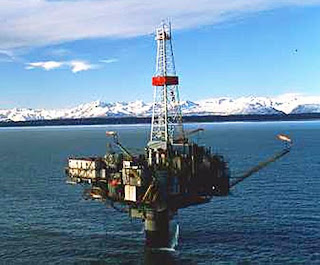 Unocal Monopod platform in Cook Inlet (Cook Inlet Oil and Gas )
 Fields (oil is green, natural gas is red) in Cook Inlet, Alaska (Alaska Department of Natural Resources via Cook Inlet Oil and Gas )
In 1958 natural gas was discovered in the Kenai Peninsula, and by 1962 was supplying gas to Anchorage, 85 miles away. There was sufficient natural gas available that, in 1969, a liquefied natural gas (LNG) plant was built and began shipping LNG to Japan, the first such export from the US to Asia. By 2009 some 1300 tanker loads, with an original deadweight capacity of 36,896 tons, had been shipped through that train.
There were two original tankers on the run, the POLAR ALASKA and the ARCTIC TOKYO, partially made of balsa wood and invar steel and they made the twenty-one day round trip until 1993, when they were replaced by the POLAR EAGLE and the ARCTIC SUN, each with a deadweight of 87,000 metric tons. The ships were renamed POLAR SPIRIT and ARCTIC SPIRIT at the end of 2007, when the registration was moved from Liberia to the Bahamas. They were sold to Teekay Corporation at that time, but leased back for the duration of the project. With the declining production from the plant, the ARCTIC SPIRIT was returned to its owners in April, 2009.
The recent drop in the price for LNG on the world market, meant that the POLAR SPIRIT was returned to its owners at the end of this past April, with the end of the original charter. It now appears to be shuttling between Yokahama and the China Sea, with the last call in the US being in June. The LNG facility was mothballed at the beginning of this summer since Alaskan LNG was no longer competitive on the market.
The original two LNG carriers were renamed SCF POLAR (which left Las Palmas a couple of days ago) and SCF ARCTIC which left Point Fortin this morning.
The region has never been one of intense activity, with only a relatively few wells being drilled in any one year.
 Exploration wells drilled in the Cook Inlet region of Alaska since 1950 (Oil and Gas )
At present there are two jack-leg drills heading for Cook Inlet, with the state providing some of the funding ($30 million) for this new drilling activity.
The wells that have been drilled and brought into production in the past have produced, to date, around 1.3 billion barrels of oil, 7.8 trillion cubic ft (TCF) of natural gas and 12,000 bbl of natural gas liquids in total. At the end of June the U.S. Geological Survey (USGS) announced the results of a new assessment of the resources of the region. There is a considerable amount of coal in the region, which is likely to contain methane, and this is now included.
 Potential resources of Cook Inlet, Alaska (USGS )
The excluded region in the above graphic shows the coal that lies below 6,000 ft, and is considered unlikely to hold any gas. In addition to this coalbed methane, the USGS re-evaluated the likely volumes that are held in the sandstone and conglomerates that have, to date, been the host rocks for the oil and gas that has been extracted. Finally the USGS assessed the potential of tight sands in the region to hold technically recoverable volumes of gas.
As the recent experience with natural gas has shown, just because a resource exists, and can be recovered, does not mean that it will make sufficient money to justify the investment in the extraction. Thus the USGS can only say that there is a significant likelihood of oil and gas being present and recoverable, without bringing the costs and price of the fuels on the market into the discussion, and thus defining whether the resource is, or will be a reserve, or not.
Because the volumes are estimates, they vary from there being a 95% chance that there is some 5 Tcf of natural gas available, to a 5% chance that there is 39 Tcf of natural gas present. In the same way they estimate that there is a 95% chance of 108 million barrels of oil (mbo) being present, while there is a 5% chance that there might be as much as 1.3 billion barrels. Unfortunately current prices are not necessarily that favorable to much exploratory drilling to validate some of those numbers, though obviously they are favorable enough to convince the Governor to put up some money.
But another part of the reason for this lack of interest has been because of the much larger volumes of Alaskan oil that lie considerably further North, in the region known as the North Slope, which I will discuss next time. But that is beginning to run out, and there are other problems that are apparent, so the resources further South may have thus become more attractive.
Incidentally the mothballing of the LNG plant is leaving Anchorage with a wee bit of a problem. Until this year the facility has acted as a transient storage facility from which, in periods of high demand (such as the depth of winter) gas could be temporarily withdrawn to make up temporary shortages between demand and supply from the wells in the field. That has now gone.
 Natural oil seep, Oil Creek, Alaska (David Page )
These seeps occur both on and offshore, and as happened in the rest of the country, it was these seeps that brought prospectors to the region, and where the first wells were drilled.
 Location of natural seeps along the Alaskan coast. (after David Page and the Copper River and Northwestern Railway )
It is pertinent to note that the creeks shown above are productive salmon spawning grounds, though it was the oil that led to early development.
The first producing field was at Katalia on the Gulf of Alaska. Discovered in 1902, it produced 154,000 bbl of oil before the refinery burned in 1933.
 Early Drilling rig at Katalia in Alaska (Cook Inlet Oil and Gas )
The larger fields in and around the Cook Inlet began production with the development of the Swanson River field in 1957. The first Alaskan pipeline was built in 1960 to carry oil from there to the Nikiski refinery (which later supplied the fuel to the International Airport in Anchorage. The Cook Inlet fields peaked in oil production, at 227,400 bd, in 1970. The largest oil field in the region was the McArthur River field, discovered in 1965, but while discoveries continue to be made, the majority of the wells are now past their prime, and will need significant work to be brought back into production. The more recent developments were offshore, with a considerable change in structure from that of the early days.
 Unocal Monopod platform in Cook Inlet (Cook Inlet Oil and Gas )
 Fields (oil is green, natural gas is red) in Cook Inlet, Alaska (Alaska Department of Natural Resources via Cook Inlet Oil and Gas )
In 1958 natural gas was discovered in the Kenai Peninsula, and by 1962 was supplying gas to Anchorage, 85 miles away. There was sufficient natural gas available that, in 1969, a liquefied natural gas (LNG) plant was built and began shipping LNG to Japan, the first such export from the US to Asia. By 2009 some 1300 tanker loads, with an original deadweight capacity of 36,896 tons, had been shipped through that train.
There were two original tankers on the run, the POLAR ALASKA and the ARCTIC TOKYO, partially made of balsa wood and invar steel and they made the twenty-one day round trip until 1993, when they were replaced by the POLAR EAGLE and the ARCTIC SUN, each with a deadweight of 87,000 metric tons. The ships were renamed POLAR SPIRIT and ARCTIC SPIRIT at the end of 2007, when the registration was moved from Liberia to the Bahamas. They were sold to Teekay Corporation at that time, but leased back for the duration of the project. With the declining production from the plant, the ARCTIC SPIRIT was returned to its owners in April, 2009.
The recent drop in the price for LNG on the world market, meant that the POLAR SPIRIT was returned to its owners at the end of this past April, with the end of the original charter. It now appears to be shuttling between Yokahama and the China Sea, with the last call in the US being in June. The LNG facility was mothballed at the beginning of this summer since Alaskan LNG was no longer competitive on the market.
the plant received needed license extensions last year, but was not able to get a satisfactory price for their LNG. . . . . . business case does not support continuing exports at this time.
The original two LNG carriers were renamed SCF POLAR (which left Las Palmas a couple of days ago) and SCF ARCTIC which left Point Fortin this morning.
The region has never been one of intense activity, with only a relatively few wells being drilled in any one year.
 Exploration wells drilled in the Cook Inlet region of Alaska since 1950 (Oil and Gas )
At present there are two jack-leg drills heading for Cook Inlet, with the state providing some of the funding ($30 million) for this new drilling activity.
The wells that have been drilled and brought into production in the past have produced, to date, around 1.3 billion barrels of oil, 7.8 trillion cubic ft (TCF) of natural gas and 12,000 bbl of natural gas liquids in total. At the end of June the U.S. Geological Survey (USGS) announced the results of a new assessment of the resources of the region. There is a considerable amount of coal in the region, which is likely to contain methane, and this is now included.
 Potential resources of Cook Inlet, Alaska (USGS )
The excluded region in the above graphic shows the coal that lies below 6,000 ft, and is considered unlikely to hold any gas. In addition to this coalbed methane, the USGS re-evaluated the likely volumes that are held in the sandstone and conglomerates that have, to date, been the host rocks for the oil and gas that has been extracted. Finally the USGS assessed the potential of tight sands in the region to hold technically recoverable volumes of gas.
As the recent experience with natural gas has shown, just because a resource exists, and can be recovered, does not mean that it will make sufficient money to justify the investment in the extraction. Thus the USGS can only say that there is a significant likelihood of oil and gas being present and recoverable, without bringing the costs and price of the fuels on the market into the discussion, and thus defining whether the resource is, or will be a reserve, or not.
Because the volumes are estimates, they vary from there being a 95% chance that there is some 5 Tcf of natural gas available, to a 5% chance that there is 39 Tcf of natural gas present. In the same way they estimate that there is a 95% chance of 108 million barrels of oil (mbo) being present, while there is a 5% chance that there might be as much as 1.3 billion barrels. Unfortunately current prices are not necessarily that favorable to much exploratory drilling to validate some of those numbers, though obviously they are favorable enough to convince the Governor to put up some money.
But another part of the reason for this lack of interest has been because of the much larger volumes of Alaskan oil that lie considerably further North, in the region known as the North Slope, which I will discuss next time. But that is beginning to run out, and there are other problems that are apparent, so the resources further South may have thus become more attractive.
Incidentally the mothballing of the LNG plant is leaving Anchorage with a wee bit of a problem. Until this year the facility has acted as a transient storage facility from which, in periods of high demand (such as the depth of winter) gas could be temporarily withdrawn to make up temporary shortages between demand and supply from the wells in the field. That has now gone.
Read more!
Saturday, August 13, 2011
Delaware combined temperatures
The last post in this series looked at the temperatures for Maryland and so, moving up along the coast, the next stop is Delaware.
 Delaware USHCN stations (CDIAC)
Given the small size of the state, I thought it might also be interesting to compare the results with those for the GISS station in Washington D.C., since the latter would otherwise be left out. They are at about the same latitude, and of somewhat similar elevation, differing only in the size of their populations.
 Temperatures as reported for the GISS station in Washington D.C. (GISS )
Given the built-up nature of the area around Wilmington there could be some debate as to the relative population sizes about the various stations, but for the moment I will accept the values from the citi-data sites that I have used to date. (The question is raised particularly regarding the Newark University Farm, which GISS considers to lie within metropolitan Wilmington).
It turns out that Washington is, on average, about 2.76 deg F hotter than the average for Delaware, though the difference has changed, with a steady increase until around 1980, and a fall thereafter.
 Difference between the temperature reported for the GISS station at Washington DC and the USHCN average homogenized temperature for Delaware.
Looking at the overall change in temperature over time for Delaware alone, there is still that drop in temperature that occurs between around 1948 and 1965:
 Average temperature for the USHCN stations in Delaware after homogenization.
Before homogenization, however, looking at the Time of Observation adjusted raw data, the trend is not as significant:
 Average temperature for the USHCN stations in Delaware raw data after correction for time of observation (TOBS).
The temperature drop from around 1950 to 1965 is still present, but the overall temperature increase has fallen from 1.9 deg F per century down to 0.5 deg F per century.
Delaware is the second smallest state (after Rhode Island) and is only 100 miles long, while 30 miles wide. It stretches roughly from 75 deg W to 75.75 deg W, and from 38.5 deg N, to 39.8 deg N. The mean latitude is sensibly 39 deg N, the average of the USHCN stations is 39.3 deg N (D.C. is at 38.85). The state elevation runs from sea-level to 137 m with the mean at 18.3 m. The average of the USHCN stations is at 28.6 m.
The small number of stations makes the correlation coefficients of little real value, but they are included for consistency. It will be interesting to see how these numbers fit in when I compile the overall statistics.
 Change in average station temperature in Delaware as a function of latitude.
 Change in average station temperature in Delaware as a function of longitude.
Because of the relatively small change in elevation for the different stations, the correlation with elevation is not as evident here.
 Change in average station temperature in Delaware as a function of elevation.
When I looked at the TOBS data available there is insufficient recent information to provide a realistic plot of temperature against local population unfortunately, but I’ll include the plot for consistency.
 Change in average station temperature in Delaware as a function of population around the station.
It is clear in Delaware, as elsewhere, that the homogenization of temperature data, has led to an increase in reported temperatures with time.
 Increase in temperature from the TOBS data to the reported homogenized temperatures for the stations in Delaware.
Read more!
Thursday, August 11, 2011
OGPSS - North Dakota and the Bakken shale
Nick has pointed out that the chart I used last time, in writing of the production in the deep waters of the Gulf is out of date. North Dakota is heading for second place behind Texas, having passed Oklahoma, and has the ability to pass Alaska in a few years. In May the state was averaging a production of 361 kbd of oil, and 361 bcf of natural gas, from a total of 5,570 wells (all three figures being all-time highs). Gas flaring, at the moment, is at around 29%. The current rig count is at 183 and also an all-time high. So where is all the excitement? It is not in shallow gas given that, as the Director of the Department of Mineral Resources has noted::
 OOIP estimates by county (North Dakota DMR)
The state has also produced some three-dimensional models of the formations in the region around Williston, which is where some of the most productive wells are found.
 Region of North Dakota that is modeled. (ND DMR ) The sides of the square cover 135 miles.
By developing the model it is possible to look both at the section showing the location of the productive beds in the region. Since the Department covers other valuable minerals beside oil and gas, they are also shown in the section:
 Section through the ND geology (ND DMR )
The Bakken lies at a depth of around 11,500 ft with the additional need for rigs to drill 20,000 ft coming from the use of horizontal drilling along the formation, which is typically only around 150 ft thick. One of the advantage of the model is that it can be used to generate a view of the Bakken itself, with the overlying ground removed. This also helps show that, while the above section shows the beds lying in a syncline, where oil might be expected to migrate out and up the sides away from the central dip, there is a central anticline where oil could be trapped, and the structure is not smooth. (Bear in mind also the scale of the model, so that small traps in the field are not picked up at this level. ) The structure of the shale beds themselves also make it less sensitive to geological modifications which drive oil migration, though obviously not completely or else there would be little oil flow to the well.
 Model of the Bakken formation around Williston (ND DMR )
The dominant feature that runs relatively North-South through the center helps then explain the location of many wells drilling into the reservoir.
 L:ocation of wells in the modeled region of North Dakota (ND DMR )
While the formations have been known for some time it was only with the development of horizontal wells, and fracking capabilities, that the opportunities to extract the oil became viable. To borrow a picture from that earlier post by Piccolo (H/t Gail)
 Change in Bakken production with the introduction of horizontal wells and Fracing (TOD)
As the number of horizontal wells has grown one finds, as I noted above, that 20,000 ft of drilling will include perhaps 9,000 ft of horizontal well in the formation itself. Such a well, as for example the Credo Petroleum well that is cited, may initially produce 1,267 bd of oil and 1.24 mcf/day of natural gas.
However one of the concerns that has been expressed, both by Art Berman, and later myself, has to do with the long-term production rate from long horizontal, frac’ed wells in shale, and it is therefore instructive to see the information that is now available on a typical well, which has been compiled by the ND DMR.
 Typical Bakken well production (ND DMR )
At the time of the presentation (last year) there was still a large proportion of the gas being flared.
 Gas flared as a percentage in ND (ND DMR )
Since then, as I noted at the start of the piece, the amount flared in May of this year has risen to 29%.
There is a more than adequate array of pipelines to handle the fuel that is being produced, at the moment it is the oil that is the critical, and valuable component. But even with a projection that the state will see about 2,000 wells a year being drilled over the next few years, with the expectation that the field will last some 20 years, the overall production is not expected to increase much beyond the levels that it is now attaining. This is because of the relatively rapid drop in well production, for which there is now a considerable data base. That doesn’t stop some from projecting, however, that the field can increase in production to levels as high as 1 mbd or so. That would, of course, include production from Montana and Canadian parts of the Bakken, which I have not discussed here.
One point that should be noted is that the lease rates for Bakken in North Dakota are quoted as being around $7,000 to $8,000 per acre, while those in Montana are reported to be considerably less. To date there has not been that much activity in Montana, though with time this will change. Already permit numbers are rising, and there has been some success to equal that in North Dakota.
At present, however, most of the rigs (170 to 10) remain on the North Dakota side of the border. That too will change, with time.
Overall the Bakken is likely to see further increases in production as the areas being drilled expand, but with the relatively short life of the well at significant levels of production, it is harder to see the higher levels of production overall that others have cited, and one also has to remember that is often the sweetest spots that get drilled first.
North Dakota Shallow gas exploration is not economic at the current price.The answer lies in the Bakken and Three Forks with rigs that can drill more than 20,000 ft being the most actively employed. The Bakken has already been discussed in an earlier post at The Oil Drum and I don’t really want to repeat much of that information, and so this presentation will, perhaps, rely a little more on visuals. The Bakken and Three Forks partially lie in Western North Dakota, and the Department of Mineral Resources (DMR) for the state, has shown how the total Original Oil In Place (OOIP) estimates vary from county to county within that region.
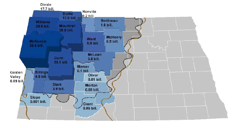 OOIP estimates by county (North Dakota DMR)
The state has also produced some three-dimensional models of the formations in the region around Williston, which is where some of the most productive wells are found.
 Region of North Dakota that is modeled. (ND DMR ) The sides of the square cover 135 miles.
By developing the model it is possible to look both at the section showing the location of the productive beds in the region. Since the Department covers other valuable minerals beside oil and gas, they are also shown in the section:
 Section through the ND geology (ND DMR )
The Bakken lies at a depth of around 11,500 ft with the additional need for rigs to drill 20,000 ft coming from the use of horizontal drilling along the formation, which is typically only around 150 ft thick. One of the advantage of the model is that it can be used to generate a view of the Bakken itself, with the overlying ground removed. This also helps show that, while the above section shows the beds lying in a syncline, where oil might be expected to migrate out and up the sides away from the central dip, there is a central anticline where oil could be trapped, and the structure is not smooth. (Bear in mind also the scale of the model, so that small traps in the field are not picked up at this level. ) The structure of the shale beds themselves also make it less sensitive to geological modifications which drive oil migration, though obviously not completely or else there would be little oil flow to the well.
 Model of the Bakken formation around Williston (ND DMR )
The dominant feature that runs relatively North-South through the center helps then explain the location of many wells drilling into the reservoir.
 L:ocation of wells in the modeled region of North Dakota (ND DMR )
While the formations have been known for some time it was only with the development of horizontal wells, and fracking capabilities, that the opportunities to extract the oil became viable. To borrow a picture from that earlier post by Piccolo (H/t Gail)
 Change in Bakken production with the introduction of horizontal wells and Fracing (TOD)
As the number of horizontal wells has grown one finds, as I noted above, that 20,000 ft of drilling will include perhaps 9,000 ft of horizontal well in the formation itself. Such a well, as for example the Credo Petroleum well that is cited, may initially produce 1,267 bd of oil and 1.24 mcf/day of natural gas.
However one of the concerns that has been expressed, both by Art Berman, and later myself, has to do with the long-term production rate from long horizontal, frac’ed wells in shale, and it is therefore instructive to see the information that is now available on a typical well, which has been compiled by the ND DMR.
 Typical Bakken well production (ND DMR )
At the time of the presentation (last year) there was still a large proportion of the gas being flared.
 Gas flared as a percentage in ND (ND DMR )
Since then, as I noted at the start of the piece, the amount flared in May of this year has risen to 29%.
There is a more than adequate array of pipelines to handle the fuel that is being produced, at the moment it is the oil that is the critical, and valuable component. But even with a projection that the state will see about 2,000 wells a year being drilled over the next few years, with the expectation that the field will last some 20 years, the overall production is not expected to increase much beyond the levels that it is now attaining. This is because of the relatively rapid drop in well production, for which there is now a considerable data base. That doesn’t stop some from projecting, however, that the field can increase in production to levels as high as 1 mbd or so. That would, of course, include production from Montana and Canadian parts of the Bakken, which I have not discussed here.
One point that should be noted is that the lease rates for Bakken in North Dakota are quoted as being around $7,000 to $8,000 per acre, while those in Montana are reported to be considerably less. To date there has not been that much activity in Montana, though with time this will change. Already permit numbers are rising, and there has been some success to equal that in North Dakota.
Brigham Exploration, one of the most aggressive in Montana, recently unveiled five wells there ranging from 909 boe/d to 2,962 boe/d, the latter volume a "record for the state," Pritchard said. The five wells averaged 1,579 boe/d.
At present, however, most of the rigs (170 to 10) remain on the North Dakota side of the border. That too will change, with time.
Overall the Bakken is likely to see further increases in production as the areas being drilled expand, but with the relatively short life of the well at significant levels of production, it is harder to see the higher levels of production overall that others have cited, and one also has to remember that is often the sweetest spots that get drilled first.
Read more!
Subscribe to:
Posts (Atom)


