OGPSS - The East Texas field develops

Last week I discussed the start of oil production in the United States, and the evolution of the Appalachian fields which, for a while, were the most productive in the world, but which are now largely depleted. It was possible, however, to take the odd well to show that where production is largely managed, so the ultimate recovery from a reservoir can be continued for decades.

Appalachia was displaced as the production leader by the East Texas oilfield. This field, with oil held in the Woodbine sandstone, was first discovered in 1927, though there was no significant production until the end of 1930.

The first oil leaving the field went in thirteen tank cars of 10,000 gallons each to the Sinclair refinery in Houston. Later, in December 1930 Ed Bateman, a Fort Worth promoter who ran a poor-boy operation called Bateman Oil Company, completed a well ten miles to the northwest of the Bradford No. 3 in the E. G. Sevier Survey, Rusk County. It was the Lou Della Crim No. 1, and it flowed 22,000 barrels of oil per day from 3,653 feet. With four producing wells at the end of 1930, East Texas field reported a yearly production of 27,000 barrels of oil and no gas.

This led to an immediate frenzy of drilling, which in turn led to the first controls on well production, with the Texas Railroad Commission preceding OPEC by decades in the moves that it made to define targets for production. There are a couple of other relevant stories about the field, and so it is a useful second stop as we look at the evolution of American oil production.

There are (as with many things) rather a lot of oil and gas wells in Texas. In 2005 there were still 66,951 active gas wells and 151,605 active oil wells.

Producing wells in Texas in 2005 (Bureau of Economic Geology)

The state, and surrounding regions, have a number of different oilfields within their borders, with East Texas being where you might think.

Major Texas hydrocarbon basins (Bureau of Economic Geology)

A section along the B-B’ line gives some idea of the formations, and will be a useful guide when I come to talk about reservoirs associated with salt domes later in the series, although they were the cause of the first great Texas oil rush at Spindletop.

Section showing the rock structure in East Texas(Bureau of Economic Geology)

East Texas was not the first oil field in Texas to be brought into production,nor the mmost famous. That resides with Spindletop down near Beaumont in Southeast Texas which is remembered as the most dramatic, when it blew back in 1901.

On January 10, at around 10:30 a.m. the Lucas Gusher at Spindletop blew. The oil spray, which could be seen for ten miles, was fully six inches across and rose to over 200 ft above the derrick. . . . . .

Nine days and 800,000 barrels later, they cut the gusher off.

Over 285 active wells were drilled into the formation under Spindletop Hill. But the field rapidly declined in production over the next five years, although it was a major contributor to America being able to reach a production of 1 mbd in 1919.

The overabundance of wells at Spindletop led to a rapid decline in production. After yielding 17,500,000 barrels of oil in 1902, the Spindletop wells were down to 10,000 barrels a day in February 1904.

In 1926 there was a second surge in production, which was more controlled and gave the field peak at 21 million barrels in 1927 (out of a total field production of around 153 million barrels), but this had petered out by 1931, just as East Texas was surging. Spindletop is credited with being the first well to use drilling mud, rather than water, as the cooling and transportation fluid to get the cuttings out of the hole, while keeping the hole itself stable.

The production potential of the Woodbine sandstone in East Texas, in contrast, was greatly helped because the oil lay over water, and this underlying water helped to sustain the driving pressure that helped keep the wells in production over longer time intervals. Of course that only holds true to a degree. And back in 1931 there was little constraint on how close wells could be.

Wells at Spindletop in 1902 (Spindletop- Gladys City Boomtown Museum )

This led to a great rush to bring wells into production, given that the this production was governed by what is known as “the rule of capture.” This, in essence said that if the well came into your well by flowing out from under your neighbors yard, then that was just tough for him/her, providing that your well remained on your land all the way. That ruling came about ultimately through an 1889 Pennsylvania Supreme Court decision. However it should be noted that the well has to remain on your property. There was a considerable scandal in East Texas in 1962 when it was discovered that some wells had “bent” so that instead or remaining on the owners property they ended on someone else’s lease, and took that oil. That is not allowed, and became a scandal when the scale of the mischief was discovered.

It was learned that operators had drilled slanted holes from barren acreage beyond the limits of the field back into the Woodbine formation, tapping into productive leases owned by major companies. During a series of investigations, inspectors found 380 deviated wells in East Texas field and shut them down. An estimated $100 million worth of oil was stolen over several decades from legal owners. Many of the oil pirates were leading citizens of East Texas communities.

Yet this wasn’t the greatest problem with the field. So productive did the wells become that the amount of oil available saturated the market available, and within months the price of oil had plummeted. It began the year at $0.99 a barrel, but by July was down to $0.13 a barrel, and something had to be done. The industry answer had been to increase production at individual wells as the price fell, but the problem with increasing production can perhaps be illustrated by example.

If you take a cup of black coffee and very carefully pour cream into the cup over the back of a spoon at the level of the coffee you can “float” the cream on top of the coffee. (And if you are of that frame of mind you can do this will various different alcohols in a bar). If you put a straw into the cream and suck gently you can pull most of the cream into the straw, and thence into your mouth (production) without getting any coffee. But if you suck too hard then the coffee comes up through the cream into the straw and you can’t reverse the situation.

So it is with an oil well. If there is water under the oil (as there is in East Texas) then sucking too hard (relatively) will pull the underlying water up into the well rather than the surrounding oil. The process is called “coning” and can be illustrated.

Water coning (Schlumberger )

Obviously this is not desirable, but if the alternate to pumping like crazy to get all the oil out from under your derrick before it all flowed to your neighbors was to lose the production to them, folk just hoped coning wouldn’t happen to them. The combination of damage to the field, and the glut of oil that this produced had an immediate effect on price. Something had to be done, and it was.

On August 17, 1931, the governor ordered the Texas National Guard and Texas Rangersqv into the ten-month-old field to shut in all of its 1,644 wells and to maintain order. The field resumed production on September 5, 1931, under a new proration order that limited its production to 400,000 barrels of oil per day, permitting each well 225 barrels and giving no consideration to its potential or to the characteristics of the lease. New wells came on line, and by October allowables were reduced for each one to 165 barrels per day.

And it was from those days that the Railroad Commission of Texas acquired its power. But that is a sufficiently interesting story that I will go into it more next time.

In the interim, let me leave you with this thought. The production of oil in Texas peaked in 1972, and in March of that year the Railroad Commission lifted restrictions on produced volumes for individual wells.

The peak in Texas oil production (U of Texas )

However the profile of that peak, and the resulting decline (in which period there were no longer regulatory restrictions) has, as Westexas has noted, been similar to the decline of other fields. It thus allows modeling and a prediction of future oilfield production post peak. But that too is a topic best left for another day.

A similarity in peak profiles (Westexas )

Arkansas - the homogenized data results

Unfortunately I still do not have access to the CDIAC server showing the information on the USHCN sites in Arkansas, so as I discussed last time I have obtained the information from the surface stations site and then downloaded the various station temperatures from the GISS site. Unfortunately this does not include the TOBS data, only that homogenized before being published. There are some problems with that homogenization, which really requires both sets of data to illustrate, but I’ll leave that for now, just to do an initial review of the Arkansas initial data set, and to look at the population data.

There are only 15 USHCN stations, and one GISS station (Fort Smith) on the list, so that the initial work was not that demanding.

Fort Smith GISS temperatures

The difference between the GISS station and the average of the USHCN curves uses the same data set as in the rest of the series:

Difference between the GISS temperature and the average of the homogenized station data for the USHCN stations in Arkansas

The shape of the curve seems to show an increasing difference through about 1948, and then a decline since that time. Given the switch in some series to only using data after 1948 this is slightly curious.

Turning to the overall change in temperature of the state over the century, and now using the homogenized data (hence the purple) rather than the TOBS raw data, the line still does not show very much of an increase over the past century.

Average temperature change in Arkansas over the past 115 years.

The temperature has been increasing at the rate of some 0.05 deg F per century, which is not a lot.

Arkansas is some 260 miles by 240 miles in size running from roughly 89.6 deg to 94.7 deg W in Longitude, and 33 deg to 36.5 deg N in Latitude. The highest point is at 839 m, and the lowest is at 16.7 m, with the average elevation of the state being at 198 m. The average USHCN station is at 176 m, and the GISS station is at 134 m.

Checking the populations, that of Rohwer is too small for citi-data, so I used zip area code to find 77. Fort Smith (the site of the GISS station) has the largest population of the stations.

Looking at the effects of the geography on the temperatures, beginning with the effect of Latitude.

Effect of latitude on temperature in Arkansas

There is the usual strong correlation, whereas with Longitude:

Effect of longitude on temperature in Arkansas

As has been discussed before, any correlation is likely an artifact reflecting changes in elevation.

Effect of elevation on station temperature in Arkansas

When one looks at the effect of population, using the homogenized data, rather than the TOBS data, then there is sensibly no effect of population, in fact such correlation as exists is negative.

Effect of population on temperature in Arkansas after the data has been homogenized.

OGPSS - The Appalachian Basin, simple lessons in the beginning

There are a number of different ways of getting oil from a reservoir, and, to radically oversimplify, the harder that you try to maximize the rate of production of oil from a well, then the shorter the overall life of the well will be, and there is a strong likelihood that the amount of oil, in total, that the well recovers will also decline with that increased extraction rate. This lesson, that of controlling the extraction rate from a reservoir to maximize absolute production volumes is one that Saudi Aramco practices, and because of that approach, has me quite doubtful that they will ever produce more than 12 mbd. (At least as long as the present faction of the House of Saud remains in power). To do so would hurt their absolute recoveries, and with the slower and more controlled extraction they have demonstrated that they can recover higher percentages of the total volume of oil originally present in the reservoir. It is not, however, a philosophy that is widely adopted. And yet, instead of the owners of the wells having that prescience, on occasion it has been other external forces that have driven the extraction rates from the wells, and thus controlled the length of their life and the total ultimate recoveries. The Appalachian oilfields in the United States, where much of this story began, has a history that helps illustrate some of these points.

The Oil Age is famously credited as having started with the drilling of the Drake Well in Titusville, Pennsylvania in 1859, although Ohio claims that the “First Oil Well”, was the Thorla-McKee well which was drilled and cased in oak in 1814. There is similarly a claim for the first great American oil well in Burkesville, Kentucky in 1829. I mention these as much to indicate that it was not that difficult initially to encounter oil in different parts of the country, and relatively close to the surface. The Drake well had only to extend down to 69.5 ft before it struck oil, and it made around 20 barrels of oil a day – but it was this well that opened the way to the oil industry of today.

Geological column at the Drake well site. The oil was found in the Riceville Shale (The Paleontological Research Institution)

Following on from that development, the production of oil from the nearby oilfields, first of Pennsylvania and then also into West Virginia in what became known as the Appalachian Basin dominated early American crude oil supply. :

Consider this - Pennsylvania was responsible for 1/2 of the WORLD'S production of oil until the East Texas oil boom of 1901.

Yet when we look at the map of the top oilfields ranked by proven reserves, as issued by the EIA, none of the fields in that region even appears today.

Top 100 oilfields ranked by proven reserves in 2009 (EIA)

There are two thoughts that come from this. The first is that just because an area was productive of oil at one time does not mean that it can continue to be so. And as productive fields are exhausted and production moves elsewhere the remaining oil in the field becomes less attractive as a reserve to be developed. The original Drake well at Titusville, for example, stopped producing after two years. Yet many of the wells that continued production were not produced with the tools that drive higher production today, and so tended to last much longer, but at low levels of production.

Which brings me to a second thought, which is more exemplified by wells in the Gulf of Mexico that were damaged during the Hurricanes in 2005. Until then these platforms had been producing small quantities of oil on a regular basis. But after the hurricane destruction those small quantities of oil that could be still recovered did not frequently justify the increased financial investment in extensive new drilling and repair that would have been required to re-create productive wells. And so the remaining oil in parts of the area was abandoned. Many of the wells in Appalachia ended up in a similar state.

The oil and gas fields of PA lie in the upper left (North-West) corner of the state, and are, at the moment, under much greater scrutiny again because of the natural gas that is found in the Marcellus shale that runs through the state.

Conventional Oil and gas fields in PA (PA Department of Conservation and Natural Resources )

The Marcellus is not shown on the above map, but I showed its extent in the recent post on the EIA shale gas report. Twenty-four fields are currently listed. Conditions during the oil boom at the end of the 19th Century were more intense even than the gas boom of today.

Less than twelve months ago McDonald, Pennsylvania, eighteen miles west of Pittsburgh, was a sleepy and commonplace little coal-mining town. In six months it doubled in population and became the busiest and most typical oil town in the country.

In this oil field on June 1st 1891 there were three completed oil wells. By November there were over three hundred wells in various stages, of which nearly one half were in and about McDonald.

Interestingly as Caplinger notes

Drilling and production in the United States have been governed by the price of oil, classic supply-and-demand responses to economic reality. After the initial discovery of oil at Drake’s well in 1859, prices were up to $16.00 a barrel, but high production quickly lowered the price to a fraction of this. Appalachian oil averaged $1.80 a barrel after the initial period of extremely high prices, reaching a low of 56 cents per barrel in 1892, and a high of $5.35 a barrel in 1920. Between 1859 and 1930 the price of oil in the United States averaged $1.34 per barrel. Well production in Appalachia averaged 0.6 barrels a day (the nation’s lowest), while the national average was 8.4 barrels per day.

However, Appalachia’s oil wells were the longest-lived in the country, and proved their worth in long-term production. On average, they returned 2.9 percent of their initial drilling cost per year.

Of the 600,000 wells drilled in the United States between 1959 and 1930 about half were still producing in 1930, and of these 242,000 had been drilled in Appalachia, of which 20% were dry holes and 149,000 were still producing in 1930. The average cost to drill a well in Appalachia at that time was $11,474.

Not all wells were that unproductive, although higher producers also tended to be shorter lived, (ibid)

The Funk (or Fountain) well produced 300 barrels a day for over a year before suddenly going dry. The Empire well, drilled in September of 1861, produced 3,000 barrels a day for eight months, slowing to 1,200 barrels by May 1862 before production dropped to nothing. In October of 1861, a well drilled by William Phillips on the Tarr farm on lower Oil Creek began flowing 4,000 barrels a day, probably the largest flowing well in the region’s history.

The Tarr Farm property, which once controlled the price of crude, is now long gone.

Yet not all wells ran dry that quickly. The well at the McClintock property in PA was drilled in 1861, and with long term care, and low production, is still producing 150 years later. It has, however, never produced more than 50 barrels of oil a day, and today only produces 1 - 2 bd, which is largely sold to tourists.

Unfortunately the typical well in PA was not that long lived, and the 350,000 that have been drilled, have collectively produced around 1.4 billion barrels of oil, since 1959. The Appalachian oil fields of PA oil had reached a production of 2 million barrels a year (mbpa) by 1862, and peaked at 32 million barrels a year (721 kbd) in 1892. By 1990 production had fallen to 2 mbpa again.

PA oil production (from Caplinger after Harper and Cozard

Oil production from the basin had fallen to not much more than a million barrels a year by 2001 and even though PA has no severance tax, as the following table shows, once a resource is gone . . . . .

State regulations on wells in the Appalachian Basin (Center for Rural Pennyslvania)

There was some move to looking deeper (and more expensively) at regions of the state for more resources but that has been overtaken by the developments in the Marcellus Shale. Crude oil production from PA, however, rose from 1.3 mbpa in 1997 to 3.6 mbpa in 2008.

Arkansas unavailable - hopefully just a short break on the temperature study

How long should a government run website be down? I ask because I was getting ready to download the data for the continuing study of state temperatures on Friday, intending to download the statistics from the USHCN network for Arkansas, and then compile the data, plot the curves, and write the post today. Unfortunately when I went to the site through which I go to get to where the data is:

http://cdiac.ornl.gov/epubs/ndp/ushcn/ushcn_map_interface.html

my laptop got a notice that:


Well without the data, it is hard to do any analysis. I presumed that it was a transient glitch, and went off to do other things. Came back this evening (after driving through the driving snow to Dartmouth College at noon) and got the same message, about a day later. So I went back to the NASA main website for climate change at GISS, and clicked on the:

http://cdiac.esd.ornl.gov/epubs/ndp/ushcn/newushcn.html

pointer and got the same message. (Which is also where the NOAA folk tell you to go and look).


The long way around would be to download the names of the Arkansas state stations from the Surface Stations website and then go to the GISS site, and download the data from there. Unfortunately that would only provide the homogenized data for the stations (as I found in an earlier state) not the TOBS data, which correlates better with the geographical information and population.

So I will presume that this is just a temporary problem at the site, and that, after the Easter Weekend is over, perhaps the server will be put back on line, and I can get back in business.

For now, Happy Easter, and my apologies.

Oh, a small update, I (out of curiosity) entered one of the file data references that I have used before to see if I could get around the problem that way, and got the information that:

Safari can't find the server "cdiac.csd.ornl.gov

Which was where it came from - wonder what's going on??

Drought, renewable energy, Texas, London and Florida

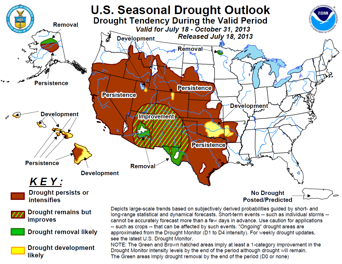
The Governor of Texas has asked the denizens of the state to pray for rain. The state has not had serious rain for months, and the drought conditions have turned severe.

The current drought conditions in Texas.

Conditions are not anticipated to get any better in the next few months. The recent predictions are that the conditions will persist in the area through July.

Predictions of the weather changes through July (NOAA )

Droughts around the world are one of the unfortunate consequences of changing weather, in much the same way as we have seen high snowfalls in other parts of the country this past winter. There will likely be cries about the underlying causes (with folks forgetting that droughts have occurred throughout history), but this post was started because of a potential event-changing occurrence.

This week Thames Water, which supplies 687 million gallons of water a day to the inhabitants of London and the immediate vicinity, was running its first water desalination plant. The region has faced droughts in the recent past as have other regions of the United Kingdom. Earlier solutions included building large water reservoirs, that at Kielder is the largest man-made reservoir in Europe. There is, however, only a certain limited amount of land that can be made available for this use, and so desalination proves an alternate way of supplying the increasing global demand for water.

In the United States droughts have threatened the viability of nuclear power stations, since the shortage of cooling water (as we recently learned again in Japan) is essential to safe plant operation. And therein lies one of the rubs to the situation. As the spokesman for Thames Water noted, the intent is not just to run the plant when there is a drought, since that is going to be too late. Rather at times of lower rainfall the plant (which can produce up to 150 million gallons a day) will pump clean water into the reservoirs, maintaining their integrity, and building up a reserve that will reduce the drought impact if it occurs. The plant was apparently completed last June at which time it was expected that it would just be used in times of drought. Within the last year that thinking has changed, and the plant is now running intermittently, partly to train operational staff, partly potentially also to help meet demand.

According to the Environment Agency, average water use is 148L per person per day in the UK and in the south-east of England it’s as high as 170L (far higher than the government target of 130L). Despite the popular perception of London as an overcast, rain-soaked city, its rainfall rate is, in fact, on a par with Rome, Dallas and Istanbul.

Schematic of the flow path through the desalination plant.

One question that I had relates to the amount of power that will be needed at Beckton. A calculation assuming that it takes 4 kWh to produce a cubic meter of fresh water, suggests that it will need a 21 MW plant. In 2009 the company CEO noted

The (20 MW) plant will be the first in the world to generate all its energy on-site, from renewable sources, including recycled cooking oil.

However the plant has been controversial, not least because although planning to use rapeseed oil, it could also burn palm oil, which is apparently cheaper. That is much more controversial. Planning permission for a second plant nearby at Southall, was refused in June 2010.

Biofuel powered stations in the UK, which includes that in the Tees Valley, where a plant burning 300,000 tons of recycled wood and specially grown wood from plantations, have had a somewhat mixed reception.

But to get back to the original idea of desalination, the largest plant in the United States is in Tampa with a maximum projected size of 35 million gallons/day, though it currently only produces some 25 million, sufficient for 10% of the region’s water needs. It went on line in 2008.

The plant uses about 44 million gallons per day (mgd) of seawater from a nearby power plant’s cooling system, which is pretreated with sand filters and a diatomaceous earth filtration system to remove particles. Reverse osmosis filters then separate 25 mgd of freshwater from the seawater. The unused concentrated seawater is diluted with up to 1.4 billion gallons of cooling water before it is discharged to the bay and that dilution is why environmental studies show no measurable salinity change in Tampa Bay related to plant production.

Which brings us back to Texas. In the latest report on desalination in the state, two possible developments are cited. There is a plan to install a 2.5 million gallon a day plant at Brownsville and a 1 million gallon a day facility on South Padre Island. Unfortunately the South Padre Island initiative failed in a bond election last year, and its future is considered doubtful. Meanwhile the Brownsville Public Utilities Board is considering combining a renewable energy source (shades of the UK) into the plant, in order to leverage funding, and possibly qualify for DOE funds.

But in the meantime, as the discussion continues, the drought gets worse. The discussions started with an initiative in 2002. As those in Texas may find out the hard way, waiting until the crisis is upon them makes it too late to construct the solution that might have helped. It appears that those in the UK and Florida were just a little more prescient. It might be noted that the initial planning for the Florida plant started in 1996.

The rising number of earthquakes in America, not Iceland

This is just a short post drawing attention to a couple of things that are starting to look a little odd. The first was the subject of a post over at Chiefio’s website pointing out that there has been a recent doubling in the number of earthquakes per day along the Western coast. This led him onto a piece that suggests that the recent activity might be a pre-cursor to a volcanic eruption near Hawthorne, Nevada – since there have been over 500 of these quakes in that area. And if one goes to the USGS site that maps their location and strength, the latest image shows that activity is still ongoing.

Recent earthquakes in the Hawthorne area (USGS )

The concentration of activity around a fixed point argues more for volcanic activity than it does a growing risk of a major earthquake. However if one looks at the region in general there is also a lot of activity along the major fault lines through California. However that tends not to be as focused, suggesting that the normal movement along the faults is continuing, though intensified just south of the border.

Recent Earthquakes on the west coast (USGS)

The two phenomena may well be separate. Generally I look for a lack of earthquake activity along a fault line as an indicator that the fault is not moving in that region, and thus stress is building up, and a larger quake will be required at some time in the future to relieve that greater stress. And in that regard it is the zone without the current quakes along the fault path that is more worrying to me than the zones where there is a lot of quaking, and thus movement.

In contrast it is the focusing of lots of earthquakes in a small area that suggests that the cause of the quakes might be more due to volcanic activity. Though one really also needs the relative vertical location of the epi-centers to determine whether magma is moving towards the surface, which is generally a warning of something in the offing.

The other thing that has me a little puzzled is the opposite situation. I have been monitoring the quakes in Iceland since the eruption last year, as reported by the Icelandic Met Office, and recording all those quakes that exceed magnitude 3. (At the bottom of this post. I note that after seeing about a hundred quakes in the past year, there hasn’t been one (greater than 3) since March 12th. Which is kinda odd.

The combination of the two events may or may not be related, we will have to see how things progress, but it is worth taking note of and keeping a closer watch to see what happens next.

OGPSS - an explanation as to where these talks go next

One of the problems in trying to project future demand and supply of oil and the other fossil fuels is that the decisions on their availability and use are often controlled by factors other than just their geological availability. Yet, at the same time, fuels cannot be created out of thin air (or empty rock) nor can viable technologies be created similarly, purely by having by the prevailing governing bodies pass the appropriate legislation (see, for example, cellulosic ethanol production). If fossil fuels are to be brought to market in a timely manner there are certain basic steps that have to have occurred.

The first step is that the deposit of whatever type has to have been found and identified. Thus, when folk discuss the shortfalls that are inevitably coming in the supply of crude oil, the first indication of this that is made, is usually the decline in the discovery of sufficient new oil in reservoirs to replace that which is being removed. And so, when the question is raised as to whether we are going to run out of oil, and if so when, the first place to look is to see what resources remain that could be counted as a future reserve for production.

And in that definition lies the first of the stumbling blocks that many commentators fail to recognize in writing about the future availability of fuels. It is a point that I made in my discussion of shale gas, namely that while there may be a lot of it out there, at present the volumes that are commercially producible are, in total, significantly less than the total volume (perhaps as little as 7% ). The total volumes that exist in the various fields are considered the resource (i.e. in this case 862 Tcf of natural gas), while the amount that can be commercially extracted is considered the reserve (in this case 60 Tcf). Confusion over the relevant values in each category, and the conditions under which volumes switch from one category to the other have been part of the debate on the glohal energy future that has, on occasion, bubbled up in places like The Oil Drum.

So if I am to develop a valid picture of where the world future is going in terms of the fossil fuels that will continue, in large measure, to power it over the next 20 years, it is important to look at the underlying resources that are available, and whether or not they can be considered reserves. And in many cases that is a relatively easy initial assessment since the volumes in question are already being produced, or are in process of being so.

But in that process there is another, somewhat controversial, number, and that is the rate at which production from a field will decline over the time that the fuel is being extracted. Back in 2009 when I wrote the initial tech talk explaining some of the reasons for this decline in an oilfield, the assumed value for this decline rate was on average 4% per annum, yet there are fields which have declined much faster than this. For example production from the Cantarell field in Mexico fell more than 75% between 2004 and 2010, with decline rates reaching more than 12% per year. Mexico has not been alone in seeing production collapse rates of this level, and yet the impact of declining production from existing fields, and the resulting need to replace it, is a factor that is not fully recognized, yet must be in any rational discussion of future conditions. If, for the sake of example, we accept that global oil production today is 88 mbd, a global decline rate average of 4% in production from existing wells per year, will require that, just to maintain production, an additional 3.52 mbd of new production must be brought on line each year. If, however, the true rate of decline is, on average, 5% then this number jumps to 4.4 mbd, and if the true decline is 6% then it rises to 5.28 mbd. (And bear in mind that this does not include the anticipated increases in demand which still run at around 1.5 mbd).

Now there are countries, such as the Kingdom of Saudi Arabia (KSA), that can manage production and the opening of new developments so that there is sufficient new production in existing fields that decline rates within the field can be kept to perhaps 2%, and new fields brought on line that reverse the total decline. KSA has been relatively forthright in the past in recognizing that without such activity they would have faced declining levels of production of perhaps 800,000 bd of their total of around 9 mbd of production. The problem, of course, is that all fields are finite. Particularly when production has been running for decades, there comes a point where the volumes available have been consumed, and there is nothing left.

Conventionally that has been a steadily changing process. As I noted in that earlier tech talk, vertical wells progressively fall in production. However, in recent years the production of oil and natural gas is being increasingly supplied from horizontal wells which do not have the same changes in production geometry over time. Rather the well may continue at relatively stable production levels until the underlying water used to maintain pressure in the formation, rises to the level of the well. And at that point the decline rate becomes very steep indeed.

In passing I should note that this “watering out” of the wells, which happens in oilwell production is not the likely cause of the dramatic fall in natural gas production from shale gas wells that has been documented.

I am reviewing these points about the changes in production with time, to explain why it is very difficult to make more than very broad generalizations when one talks about oil or natural gas (or coal for that matter) production into the future, looking only at the overall numbers. The volumes of fuel that will be available are more accurately assessed from considering the individual countries from which the production is and will be coming, what the potential futures of the fields in those countries are, and the other considerations (such as imminent or ongoing civil war) that might affect field production.

What I intend therefore to do next is to start with the major oil producers, as listed in the earlier review, although not always in that order. By looking at the different fields both past, present and future, in light of existing and possible relatively novel technologies for extraction (such as, for example, burning some of the oil in place so as to help produce the rest) I will try to bring a more accurate assessment of what the future production is likely to be, and thus build up an assessment of global production as the series continues. The top three historic producers have been the United States, Russia and Saudi Arabia, and so the series will start with North America, and more specifically the United States.

But particularly in these times when the stability of some of the producing countries is becoming more questionable, external factors do have to be addressed. Unfortunately many of these changes, being political, are harder to predict. As a result, while I will include the reasons for some of the decisions I use in building this series, I will not go into those in much depth. Rather I will focus more on the likely levels of future production that might be achieved.