OGPSS - The Railroad Commission of Texas

This post originally went up last week, and in some wonder of modern technology was wiped out by Blogger, along with a lot of other posts which had gone up at about the same time. We were promised that it would be put back, it has not been. So here, as best as I can reconstruct it, is the post. My apologies for the delay and possible confusion.

When I have written about oil and natural gas production from individual wells, in previous posts, I have referred to the website of the Texas Railroad Commission as the source of my information. You might wonder why they are in charge. Well it all began back in the days after Texas first became a State, and the government wanted to encourage folk to move out into the state. Historically railroads had been built to connect existing towns and cities, but there weren’t any going West. And so, to encourage railroads to grow out west they were allowed land grants and a number of tax and other grants and incentives that would encourage rail, and the growth of towns along the track, as a result.

Now since this provided a sensible monopoly on transportation, the Texas legislature, as far back as 1853, had enacted comprehensive laws regarding the railroads. The problem was that they were not enforced, and for a number of years the railroads could charge as much as the traffic would bear. This led to many protests, particularly from farmers, and after many promises, in 1891 the Railroad Commission of Texas (RRC) was created:

An Act to establish a Railroad Commission for the State of Texas whereby discrimination and extortion in railroad charges may be prevented, and reasonable freight and passenger tariffs may be established; to prescribe and authorize the making of rules and regulations to govern the Commission and the railroads, and afford railroad companies and other parties adequate remedies; to prescribe penalties for the violation of this act and provide means and rules for its enforcement.

That created the RRC, and after some struggles, and a trip to the Supreme Court it succeeded in establishing that it had the power, which it enforced, to cut shipping rates. But how did that allow it to get into controlling the “oil bidniss”?

The simple part of the answer is that when the Commission was set up, its responsibilities included:

Determination of passenger fares, freight rates, and charges for all classes of common carriers in Texas.

As the boom in oil production began in Texas, production rates were initially high and, as I noted last time, many wells were being drilled in close proximity, with incentives (including the “right of capture”) that drove owners to produce their wells as fast as possible. And in 1931 an average of 8 wells a day was being drilled in Texas.

The result was a glut of oil on the market with prices falling from $1.10 before the Daisy Bradford #3 well was drilled (By H.L. Hunt) to $0.15 and even $0.02 a barrel on the spot market. (The Big Rich by Bryan Burrough ) Someone had to do something, and the choice pointed to “proration”. In this each well could be assigned a certain production or number of days in the month that it could produce, based on the number of wells and the amount of oil that the market was considered able to bear. But who should set the quantities.

Oil, once it is out of the ground, has to be transported and the early alternatives were either by rail car or pipeline. The rail roads were already under the RRC and in 1917 the Texas Legislature designated pipelines as “common carriers” which also brought them under the RRC. By 1919 this oversight was extended to include jurisdiction over Oil and Gas. And a new Division was born. (The agency continued to have some role in railroads until 2005, when that was completely phased out).

The RRC had unsuccessfully tried to control production earlier, and in 1931 it tried again, setting a proration order for the East Texas field of 160,000 bd at a time when it was producing half-a-million barrels. That didn’t go anywere either, but the impact on the economies of the states was becoming too great. It was the larger companies that largely argued for proration

Jacob Wolters of the Texas Company (Texaco), warned of the ruin of thousands of wells, as well as “the bankruptcy of producers, the loss of millions of dollars in revenues of the State, and the consequent increase of taxes on other sources in order that the public schools, higher institutions of learning, eleemosynary institutions and the departments of the State may continue to function.”

Up in Oklahoma City the city council had passed a law that restricted oil wells to one per city block, and their attempt to close wells was so challenged that the Okahoma Governor, William Murray, declared martial law and closed the wells, initially for a day. This in turn led him to place the 3,106 oil producing wells in Oklahoma under martial law from August 4, 1931 until April 1933.

Down in Texas, as Bryan Burroughs notes, H.L. Hunt and other large producers urged the Texas Governor to follow suit.

On August 16, declaring East Texas oilmen to be in open “rebellion” agaist the site, he declared martial law and sent in the National Guard to shut down the oil field.

It was re-opened three weeks later, but with individual wells limited to only producing 225 bd. As these controls began to limit production in the face of growing demand so the price stabilized and slowly began to creep up. By 1933 it had reached $0.99 before falling again. A “hot oil” market was making it too lucrative to flout the law and smuggle oil, and this led to the “hot oil wars.”

To enforce the proration limits the Texas Legislature began to pass tighter and tighter regulations giving the Railroad Commission greater powers. Further the governments of Kansas, New Mexico, Texas and Oklahoma got together to establish a common approach, out of which came the Interstate Oil Compact in 1936. At the same time the Federal Government passed the Connally Hot Oil Act giving it the power to enforce the directives of the Texas RRC in interstate commerce. The regulation of output was considered as one of the steps in increasing the estimated reserves of the East Texas field from one to five billion barrels.

From 1936 until 1972, with the exception of the War years, the RRC controlled production though proration. In this way, when the Iranian revolution in 1951 nationalized the oilfields there, Texas was able to increase production and fill the gap. It was able to do the same during the Suez Canal crisis in 1958. And then, as foreign oil became a glut on the market, the RRC cut production from the wells, down to only seven days a month in 1962. But production over time was depleting the fields. When the Arab-Israeli war broke out in 1967 production could not be brought high enough to meet demand, and in 1972 the RRC set the proration at 100%. The result was only a limited gain in volume, for American oil production had peaked. And Texas had taught the rest of the world’s oil producers a lesson, for OPEC was aborning.

The commission still monitors well production, and is a site where this information is available. The site notes that both oil and gas production and oil well completions this year are running behind last years numbers.

Coal - a new technology and another look at the TV series

Back in 2008 Robert Rapier wrote a post on using coal in the making of ethanol, in which he referred back to a post he had written in 2006 on the same subject. That earlier post said, in part:

The natural gas input into ethanol production is a serious long-term threat to economic viability. Since natural gas is a fossil fuel, and supplies are diminishing, it will put upward pressure on the price of ethanol over time. However, if the energy inputs could be produced from coal, ethanol prices would be insulated from escalating natural gas prices.

Using coal might also lessen the significance of the EROEI debate. If you take 1 BTU of (cheap) coal, and you get back 0.8 BTUs of (more valuable, liquid) ethanol, then EROEI doesn't have the same significance as when you use natural gas to produce ethanol. You converted the BTUs into a readily usable liquid form. This argument may be valid from an economic point of view, but it ignores the fact that coal is still an inherently dirty energy source. If coal remains abundant and cheap, coal economics will beat natural gas economics, but coal will increase the rate at which we put carbon dioxide into the atmosphere.

In those remarks Robert was writing about the use of coal as a power source for running the ethanol plant, as opposed to the use of natural gas. The feed stock would remain the corn that is fermented, and turned into the beer that is then distilled into the ethanol that can be used as a liquid fuel source. That process still raises the debate over fuel versus food.

In an alternative approach Celanese are now starting to build plants in China that will use coal as the feedstock, without the grain, and they claim that this technology, is a game changer.

The so-called TCX technology can convert coal, petroleum coke or natural gas to ethanol for 25 percent to 35 percent less than alternative processes, Celanese said today in presentation slides posted on its website. The cost of converting coal to ethanol is $1.50 a gallon, equal to making gasoline from crude oil costing $60 a barrel, the Dallas-based company said.

“Fuel with our ethanol technology represents a game- changer for the company,” Chief Executive Officer David Weidman said in a presentation to investors in New York.

Weidman said he is advancing a November plan to build two factories in China that will turn coal into ethanol for industrial uses. The company also may produce ethanol for fuel in China, India, Australia, Colombia and Egypt, he said.

The technology, which is still being held fairly close to the Celanese chest, appears to use some of Celanese technology for the manufacture of acetic acid and involves the gasification of the coal to syngas as an earlier step. That supply will be provided by Wilson.

The use of coal is apparently currently commercial with this technology, while using the same process with a cellulosic feedstock is apparently not as yet that far along.

The two plants will each have a capacity of 400,000 tons of ethanol (134 million gallons) and will produce industrial ethanol rather than, at this stage, the fuel for use in vehicles. In China this is a larger (at 3 million tons/year) market than the fuel market, at half that size. Both are growing at up to 10% pa and the plants are expected to help meet that growth. Fuel ethanol prices in China have been estimated at $950 per tonne.

The most recent announcement comes as China is moving to increase coal imports by perhaps as much as a million tons a week due to drought reducing the output from hydro-electric power plants. Normally the country imports around 10.8 million tons a month, although this is a steadily increasing number. Without the additional imports it is possible that the country may see significant power shortages this summer, since the drought may lower available power by as much as 30 GW.

Speaking of the loss in power I did, eventually start to watch the second episode of Coal. One of the issues in that episode was the drop-out of power that was supplied to the mine. It is one of the ways in which mines can be given a lower price for electricity, if they accept that they will be “shed” if the demand exceeds that which the power generator can supply. The episode showed how that unexpected drop out can affect the men underground. Other power problems arose at the mine because the continuous miner operator was not fully experienced and was running the machine in to take too large an amount of coal or roof rock at one time. This overloaded the switches and tripped power. The necessary methodical restart of the system slows production, since nothing can start producing coal until all the components of the system are back up and running. As they are showing producing coal is not that simple or necessarily pleasant a process.

And a small additional note. In my comment on the first episode I was not that impressed with the way that the miners were bringing down the loose overhead rock. It turns out that I wasn’t the only one unimpressed. MSHA Inspectors, who watched the show, have fined Cobalt coal – for the use of improper barring tools and procedures, as well as a number of other violations.

The series has a considerable value in showing how difficult it can be to run a small mine, and though most of my experience has been in much larger operations (both financially and in terms of seam height) there are a number of different lessons that the series shows on coal mine operation. The problems of ventilation, when the belt drive started smoking and could have caught fire, are illustrative of that, with the telling message two miners died in a not too dissimilar event not that far away.

OGPSS - The Railroad Commission of Texas update

Blogger has apparently had some problems and have, along with many other posts on other sites, temporarily deleted this post. I will give them another day, and then repost it, if they have not got it back up by then. My apologies

Louisiana USHCN state temperatures

I am beginning to think that the CDIAC had the same sort of budget cuts that affected the EIA, and that this took down the server that I have been using. (Since it is still not available). So to keep going with the foundation of the data base, until I can get the TOBS information into useful form, I am going to use the Surface Station USHCN site to get the preliminary data on the stations in Louisiana. I will then download the GISS information for the stations and proceed as I did for Arkansas. This at least will get the stations and populations established.

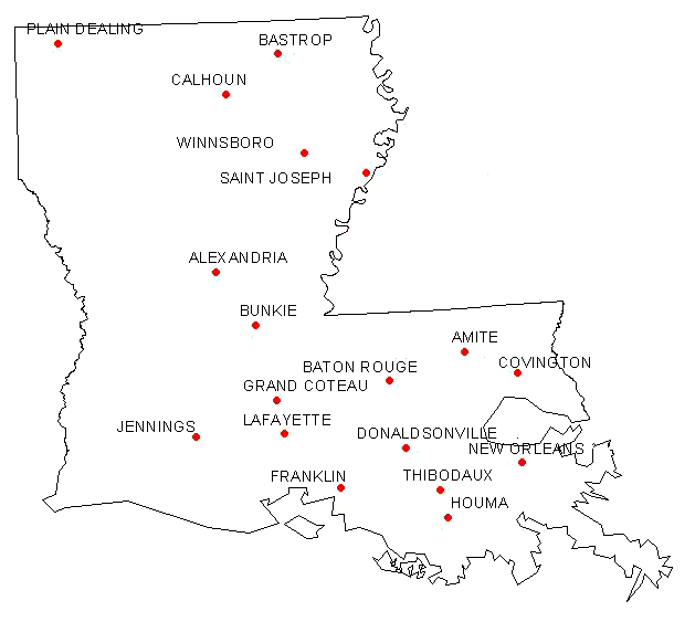
There are 18 USHCN stations in Louisiana, from Alexandria to Winnsboro, and there are two GISS stations, at Lake Charles and Shreveport, on the list. Looking for a source for the layout of the stations I find that I can get the Louisiana layout at the CO2 Science website.

Location of the USHCN stations in Louisiana ( CO2 Science)

This site calculates a trend for the mean temperature data, but for the example I chose (Alexandria) it only goes up to 2006.

Temperature trend for Alexandria LA (CO2 Science)

This is an interesting resource in that it saves me calculating the trends for the different stations. Since, at some time in the future, I had thought to move on from just the data to the trends, this will be a useful site to get that information. The question, however, is as to whether they are plotting the homogenized or raw data for the station?

Alexandria LA GISS temperature plot (GISS )

This is clearly not the same set of values, which means that there are two different homogenizations being carried out. (Note that this is recognized at the top of the CO2 Science plot). So that gives another little puzzle to look into. However, for today, it is sufficient that I have found another site that shows where the USHCN stations are in the state, so that we can get a measure of how well they are distributed.

So now I go to the GISS site (which again gives me some foreign location when I click on Louisiana) and pick Grand Coteau as being somewhere close to the middle of the state. This allows me to find the rest of the sites in the state, using the (*) facility to locate adjacent stations.

So first I download and convert the data, and discover that the GISS station at Lake Charles has only been in operation since 1948, which no longer comes as a surprise.

Lake Charles average temperatures (GISS )

On the other hand Shreveport has been reporting data since the 1880’s.

Shreveport average temperatures (GISS)

And, in passing we note that Louisiana was warmer in the 1930’s than recently. So what does the data look like (bearing in mind that I am only working with the homogenized data at the moment) ?

The difference between the USHCN data set and the two GISS stations has been steadily increasing over the years:

Difference between the average GISS station temperature and that of the average USHCN stations in Louisiana, over the past 115 years.

Looking at the actual average temperature change for the state:


Over the past 115 years the average state temperature has followed the pattern shown above for Alexandria, although the rate of temperature decrease is at a rate of around 0.05 degrees F per hundred years, which is sensibly saying that it has stayed the same. It is interesting that the visceral reaction of those who disagree is to suggest that this sample is too small, and thus meaningless – yet it is consistent with other states, and cumulatively these numbers start to gain importance.

Looking at the geographic information for Louisiana, it is a state that is 380 miles long and 180 miles wide. It runs from 89 deg W to 94 deg W, and from 29 deg N to 33 deg N. The center of the state is thus at 92.5 deg W and 31 deg N approx. The USHCN stations center on 91.6 deg W, 30.9 deg N. The GISS average is 93.5 deg W and 31.3 deg N. The average elevation of Louisiana is 30 m above sea-level, with the USHCN being at 24.4 m, and the GISS average being at 35.5 m. The highest point in the state is at 163 m.

So looking at how the temperatures are controlled by the geography, the correlation with Latitude is as expected.


And while there is a suggestion that the decline with change in longitude is significant, because of the changes in other states, I continue to consider that it, in reality, dependent to other factors.


The most likely is that of elevation, and, despite the relatively low-lying nature of the state, the correlation with elevation remains strong.


In regard to the population figures of the state, there was only Calhoun where I had to go to zip-codes to get a number. The rest had populations through the citi-data sites. And I decided, for now, to use the 5-year averages – by fixing on this before looking at future data it seems a little better than to look for a “best fit” each time.


And my apologies that these are running a little late – apart from some personal time demands, I took time this week to download all the state maps of the stations so that I will have those available for the rest of this initial series.

Power shortages in India and Pakistan

The recent publication of the EIA review of Shale Gas has caught the world’s attention, and led to the perception that the coming decades may well see natural gas become the dominant fuel. It suffers, however, a couple of disadvantages that, for some countries, make it not always the fuel of choice. India and Pakistan, have serious energy shortages as Tom Whipple recently pointed out.

In Pakistan the electricity is now turned off for 18-20 hours some days in many cities and 20 hours in rural villages. The onset of summer temperatures, shortages of fuel oil for thermal generation and falling water levels have increased the power shortfall to record levels. Without electricity to run the pumps urban water supplies quickly shut down. Without power to run the mills, exports are falling, leaving the country without money to import oil. In short we are seeing a classical downward spiral.

At the same time, in India, the domestic natural gas supply is falling, requiring increased, and more expensive imports that can only be achieved using LNG resources.

There have been discussions for years over the possibility of running gas pipelines from Turkmenistan and Iran down through Pakistan and into India to provide the natural gas needed to help. The TAPI pipeline from Turkmenistan is currently at a stage where it may be moving forward. Pakistan is ready to commit to purchasing gas by this July, but . . .

.

In the four nations’ ministerial meeting last week, both India and Pakistan had agreed to the broader aspects of the gas sales and purchase agreement (GSPA), but crucial things like the price of gas and transit fee are yet to be decided.

At present the Turkmen are expected to demand at least $7 to $7.50 per kcf, which is the price that they are getting from China. And transit fees to get the gas through Afghanistan and Pakistan to India will be added to that. (In context that is about the same price as LNG when it is currently delivered in India, and above the $4.94 to $6.42 price of domestically produced gas).

The current hope is that the pipeline will be started in 2013, with full flow to all three countries by 2016. The pipeline will have to run a thousand miles before it reaches India. And this highlights one of the problems with natural gas. It is harder to deliver than other fuels.

Oil can be put on rail cars, or tankers, as well as being piped, as can coal (though there are very few places that use pipelines to move coal). But natural gas either requires a direct pipeline, or it has to be condensed to liquid form for shipment. When large volumes are involved turning the NG into LNG requires construction of both a condensing plant at the supply end and a re-gasification unit at the customer end. Both require time to build. And one the gas is regenerated, the customer has only a limited capacity for storage, and depends on the flow coming through the delivery pipe to keep power being generated.

Coal at the other extreme used (in my youth) to be delivered to our house from the back of a horse-drawn cart. It was dumped in the street, and we shoveled it into the “coal bin” out of which we then hauled it, a bucket load at a time, into the house, and dumped it on the fire. Logistics were a lot simpler, and we kept at least a couple of weeks supply in reserve in the bin.

Times have changed somewhat, for although shovels may still dig out the coal, they now can load a hundred tons, rather than a few pounds. Rail cars can haul 120 tons apiece in unit trains of 100 cars, and power stations may use 10,000 tons of coal a day to generate 850 MW of baseload power. But the coal is often still dumped in heaps at the power station, to be used when needed. Stations will usually keep 60 to 90 days of supply on hand.

India is aware of these advantages, but has internal problems with developing enough domestic coal supplies for the power that it needs. Coal India has said that it can only deliver 100 million tons against the 330 million ton increase in demand that, over the next five years, that power stations now being built will need.

With domestic coal production floundering amid a sharp upsurge in power capacity addition, over 40,000 MW of new generation capacity could get stranded over years for want of fuel. This is close to 70 per cent of the power capacity slated to come up during the period, most of which is being set up by private developers.

With a current generation capacity of 173,626 MW, this threatens the generation of some 42,000 MW.

There is a catch with using imported coal to meet all the shortfall, because of the construction of the Indian boilers. They blend about 10% of the higher thermal content imported coal with domestic coal but there are technical problems with a higher concentration that limit how high it can be raised, as well as the additional cost factor. However new construction can be built to handle higher concentrations of imported coal, it just costs more – which is expected to be a problem in relatively poor parts of the country.

Seeing this as an opportunity, however, Adani Enterprises, an Indian coal company, has just bought the Abbot Point coal terminal in Australia, after buying coal properties in Queensland last year. Over the next five years they will bring the mines on line and be able to feed up to 50 million tons into the Indian subcontinent. It is not enough, in itself, to meet the shortfall, but it is evidence that firms in India are aware of the problem and are moving to find answers. They will do so, however, in the face of stiff competition from China. And this competition underlines the conclusions that I drew in an earlier post about the unrealistic projections of future coal use by folk such as Tad Patzek and Dave Rutledge.

Unfortunately also this does not solve the immediate problem that India faces with a current shortage of available fuel. Nor does it get Pakistan any closer to finding a short-term solution to power shortages in that country. There comes a certain point where, when warnings go unheeded, the consequences must be suffered, though sadly often not by those who weren’t paying enough attention.

Putting on blinders - the EIA Budget cuts

Pit pony wearing blinders to limit what it can see, and so make it easier to control. Horse and Man)

If you read many of the pieces that I write here you will soon notice that I am convinced that this country, and most of the civilized world, has a problem with future oil supply. That problem is getting worse rather rapidly, and this is causing the price increases that you have noticed every time you visit a gas station. It is popular, and easy, to blame the current increases on either speculators or the “evil” oil companies. While both may play a role on the edges of what is going on, the harsh reality is that prices now are largely controlled by those nations who form the OPEC partnership. Saudi Arabia, who supplies the largest portion of OPEC oil, has said that it is uncomfortable with current oil prices, since they are getting high enough that they could cause another recession. However that did not stop them from raising their prices in April and they now need the high prices to help pay to keep Saudi Arabia from seeing any of the riots that are happening to other countries. One has to know how to separate the popular myths from the actual reality.

And if legislatures at both state and national level are to make the right choices about what to do as oil prices keep going up (bearing in mind that it was a cause of the major recession in 2008) they too need to know what is really going on. There are alternate strategies for changing domestic production and alternate fuels (such as the growing supply of natural gas) that could be a significant help in the near future. Some of those that seemed to be promising, don’t always work as fast as promised, as we found out with cellulosic ethanol. They (and the rest of us who try and explain what’s happening) need to know not only what is going on, but as things change, what the effects of new rules events (such as banning drilling for a while in the Gulf of Mexico) are having on current and future supplies. It is only in this way the rational and useful steps to help get America, and the rest of the world, off this addiction to OPEC oil can be picked out, and put into place.

Because of the need to trim the Federal Budget, different Federal agencies are cutting back on the services that they provide to the public. One of the most recent has been the Energy Information Agency who have just explained in a press release, the cuts they are making. Bear in mind that this is the agency that is supposed to provide the information that I have just said that we have to have. With a tip to Gregor, the cuts that are occurring are given below, together with a comment.

Oil and Natural Gas Information
• Do not prepare or publish 2011 edition of the annual data release on U.S. proved oil and natural gas reserves.
• Curtail efforts to understand linkages between physical energy markets and financial trading.
• Suspend analysis and reporting on the market impacts of planned refinery outages.
• Curtail collection and dissemination of monthly state-level data on wholesale petroleum product prices, including gasoline, diesel, heating oil, propane, residual fuel oil, and kerosene. Also, terminate the preparation and publication of the annual petroleum marketing data report and the fuel oil and kerosene sales report.
• Suspend auditing of data submitted by major oil and natural gas companies and reporting on their 2010 financial performance through EIA's Financial Reporting System.
• Reduce collection of data from natural gas marketing companies.
• Cancel the planned increase in resources to be applied to petroleum data quality issues.
• Reduce data collection from smaller entities across a range of EIA oil and natural gas surveys.

Electricity, Renewables, and Coal Information
• Reduce data on electricity exports and imports.
• Terminate annual data collection and report on geothermal space heating (heat pump) systems.
• Terminate annual data collection and report on solar thermal systems.
• Reduce data collection from smaller entities across a range of EIA electricity and coal surveys.

Consumption, Efficiency, and International Energy Information
• Suspend work on EIA's 2011 Commercial Buildings Energy Consumption Survey (CBECS), the Nation's only source of statistical data for energy consumption and related characteristics of commercial buildings.
• Terminate updates to EIA's International Energy Statistics.

Energy Analysis Capacity
• Halt preparation of the 2012 edition of EIA's International Energy Outlook.
• Suspend further upgrades to the National Energy Modeling System (NEMS). NEMS is the country's preeminent tool for developing projections of U.S. energy production, consumption, prices, and technologies and its results are widely used by policymakers, industry, and others in making energy-related decisions. A multiyear project to replace aging NEMS components will be halted.
• Eliminate annual published inventory of Emissions of Greenhouse Gases in the United States.
• Limit responses to requests from policymakers for special analyses.

In addition to these program changes, EIA will cut live telephone support at its Customer Contact Center.

So here we are in a mess. Generally when you’re in a mess it is a good idea to understand what the mess looks like, so that you can work out how to get out of it. But now that information is not going to be locally available. Yes there will still be the information from the IEA, though it is not really comparable, and OPEC itself provides Monthly Oil Market Reports, but that is a little less independent than most, and does not cover the internal production within this country that is a valuable tool to indicate how fast we are approaching the next crisis. (And the indications are that it may well hit right around the next election). And ignoring the information (or deliberately choosing not to collect it), is not going to affect the situation from developing, only perhaps possibly it might slow our noticing, but since we go to gas stations very regularly I think that is a bit doubtful.

At some point in the future, perhaps even that soon, politicians and Administrators are going to complain “but nobody told us!!” and rush to blame the industry yet again. But the truth is that there was a group that was keeping the records, and who could tell those with the responsibility to fix it that there was a problem. And the Administration just closed it down. We will regret that lack of information and the warning messages that it would have brought.

OGPSS - The East Texas field develops

Last week I discussed the start of oil production in the United States, and the evolution of the Appalachian fields which, for a while, were the most productive in the world, but which are now largely depleted. It was possible, however, to take the odd well to show that where production is largely managed, so the ultimate recovery from a reservoir can be continued for decades.

Appalachia was displaced as the production leader by the East Texas oilfield. This field, with oil held in the Woodbine sandstone, was first discovered in 1927, though there was no significant production until the end of 1930.

The first oil leaving the field went in thirteen tank cars of 10,000 gallons each to the Sinclair refinery in Houston. Later, in December 1930 Ed Bateman, a Fort Worth promoter who ran a poor-boy operation called Bateman Oil Company, completed a well ten miles to the northwest of the Bradford No. 3 in the E. G. Sevier Survey, Rusk County. It was the Lou Della Crim No. 1, and it flowed 22,000 barrels of oil per day from 3,653 feet. With four producing wells at the end of 1930, East Texas field reported a yearly production of 27,000 barrels of oil and no gas.

This led to an immediate frenzy of drilling, which in turn led to the first controls on well production, with the Texas Railroad Commission preceding OPEC by decades in the moves that it made to define targets for production. There are a couple of other relevant stories about the field, and so it is a useful second stop as we look at the evolution of American oil production.

There are (as with many things) rather a lot of oil and gas wells in Texas. In 2005 there were still 66,951 active gas wells and 151,605 active oil wells.

Producing wells in Texas in 2005 (Bureau of Economic Geology)

The state, and surrounding regions, have a number of different oilfields within their borders, with East Texas being where you might think.

Major Texas hydrocarbon basins (Bureau of Economic Geology)

A section along the B-B’ line gives some idea of the formations, and will be a useful guide when I come to talk about reservoirs associated with salt domes later in the series, although they were the cause of the first great Texas oil rush at Spindletop.

Section showing the rock structure in East Texas(Bureau of Economic Geology)

East Texas was not the first oil field in Texas to be brought into production,nor the mmost famous. That resides with Spindletop down near Beaumont in Southeast Texas which is remembered as the most dramatic, when it blew back in 1901.

On January 10, at around 10:30 a.m. the Lucas Gusher at Spindletop blew. The oil spray, which could be seen for ten miles, was fully six inches across and rose to over 200 ft above the derrick. . . . . .

Nine days and 800,000 barrels later, they cut the gusher off.

Over 285 active wells were drilled into the formation under Spindletop Hill. But the field rapidly declined in production over the next five years, although it was a major contributor to America being able to reach a production of 1 mbd in 1919.

The overabundance of wells at Spindletop led to a rapid decline in production. After yielding 17,500,000 barrels of oil in 1902, the Spindletop wells were down to 10,000 barrels a day in February 1904.

In 1926 there was a second surge in production, which was more controlled and gave the field peak at 21 million barrels in 1927 (out of a total field production of around 153 million barrels), but this had petered out by 1931, just as East Texas was surging. Spindletop is credited with being the first well to use drilling mud, rather than water, as the cooling and transportation fluid to get the cuttings out of the hole, while keeping the hole itself stable.

The production potential of the Woodbine sandstone in East Texas, in contrast, was greatly helped because the oil lay over water, and this underlying water helped to sustain the driving pressure that helped keep the wells in production over longer time intervals. Of course that only holds true to a degree. And back in 1931 there was little constraint on how close wells could be.

Wells at Spindletop in 1902 (Spindletop- Gladys City Boomtown Museum )

This led to a great rush to bring wells into production, given that the this production was governed by what is known as “the rule of capture.” This, in essence said that if the well came into your well by flowing out from under your neighbors yard, then that was just tough for him/her, providing that your well remained on your land all the way. That ruling came about ultimately through an 1889 Pennsylvania Supreme Court decision. However it should be noted that the well has to remain on your property. There was a considerable scandal in East Texas in 1962 when it was discovered that some wells had “bent” so that instead or remaining on the owners property they ended on someone else’s lease, and took that oil. That is not allowed, and became a scandal when the scale of the mischief was discovered.

It was learned that operators had drilled slanted holes from barren acreage beyond the limits of the field back into the Woodbine formation, tapping into productive leases owned by major companies. During a series of investigations, inspectors found 380 deviated wells in East Texas field and shut them down. An estimated $100 million worth of oil was stolen over several decades from legal owners. Many of the oil pirates were leading citizens of East Texas communities.

Yet this wasn’t the greatest problem with the field. So productive did the wells become that the amount of oil available saturated the market available, and within months the price of oil had plummeted. It began the year at $0.99 a barrel, but by July was down to $0.13 a barrel, and something had to be done. The industry answer had been to increase production at individual wells as the price fell, but the problem with increasing production can perhaps be illustrated by example.

If you take a cup of black coffee and very carefully pour cream into the cup over the back of a spoon at the level of the coffee you can “float” the cream on top of the coffee. (And if you are of that frame of mind you can do this will various different alcohols in a bar). If you put a straw into the cream and suck gently you can pull most of the cream into the straw, and thence into your mouth (production) without getting any coffee. But if you suck too hard then the coffee comes up through the cream into the straw and you can’t reverse the situation.

So it is with an oil well. If there is water under the oil (as there is in East Texas) then sucking too hard (relatively) will pull the underlying water up into the well rather than the surrounding oil. The process is called “coning” and can be illustrated.

Water coning (Schlumberger )

Obviously this is not desirable, but if the alternate to pumping like crazy to get all the oil out from under your derrick before it all flowed to your neighbors was to lose the production to them, folk just hoped coning wouldn’t happen to them. The combination of damage to the field, and the glut of oil that this produced had an immediate effect on price. Something had to be done, and it was.

On August 17, 1931, the governor ordered the Texas National Guard and Texas Rangersqv into the ten-month-old field to shut in all of its 1,644 wells and to maintain order. The field resumed production on September 5, 1931, under a new proration order that limited its production to 400,000 barrels of oil per day, permitting each well 225 barrels and giving no consideration to its potential or to the characteristics of the lease. New wells came on line, and by October allowables were reduced for each one to 165 barrels per day.

And it was from those days that the Railroad Commission of Texas acquired its power. But that is a sufficiently interesting story that I will go into it more next time.

In the interim, let me leave you with this thought. The production of oil in Texas peaked in 1972, and in March of that year the Railroad Commission lifted restrictions on produced volumes for individual wells.

The peak in Texas oil production (U of Texas )

However the profile of that peak, and the resulting decline (in which period there were no longer regulatory restrictions) has, as Westexas has noted, been similar to the decline of other fields. It thus allows modeling and a prediction of future oilfield production post peak. But that too is a topic best left for another day.

A similarity in peak profiles (Westexas )