ONI and individual state temperatures

The influence that sea surface temperatures have on land temperatures and climate is an ongoing debate, and I mentioned this somewhat in my last post on this topic. However, in looking back over that post it was perhaps too general an approach to look at the impact of the El Niño events over the large scale of the West Coast, and thereon East. Given that effects were, as I showed, more regionalized and remembering that we are in a La Nina winter, I’ll just repeat the anticipated effect plot from Kumar, et al.

Impacts of a La Nina winter (after Kumar et al).

The disadvantage of using the regional average can be seen just in the US West Coast. At the upper end the season is cooler and wetter, while down in the south it is drier and warmer – the average might well be “no change.” So since we have the individual state temperatures for the period I looked at last time, I thought it might be interesting, before looking at other Oscillations, to just check how this event correlated on a more localized basis.

The ONI plot from 1950 (GGWeather )

It is logical to start on the West Coast, and given that the predicted impact this winter will be on the upper Northwest, the first comparison is with Washington State. For now I am going to use the homogenized data set, rather than the TOBS data, though I may come back later to look at how that changes things. (This is the fun of doing this without an agenda, we don’t need to have the data fit any pattern, so it is more informative to look at options).


The ONI plot overlain on a plot of Washington state temperatures.

It can be seen that while there was some correlation, in places, overall the agreement is not very good.

The other states that seem to be most impacted are the southern tier, that would include California, Arizona, and possibly New Mexico and Texas . From the regional comparison the Pacific SST effects seem to weaken somewhat once one gets over the Rockies, hence the caution as to how far we might expect the impact along the South Coast – so we shall see.

Turning first to California, recognize in the beginning that with the state being as long as it is, there are internal temperature variations along the state, Overlaying the ONI plot on the relevant part of the California temperature curve:

Relation of California temperatures to ONI temperature anomalies

My sense is that the correlation is a bit better, but still lacking. So let’s try the Arizona comparison:

Relation of Arizona temperatures to ONI temperature anomalies.

There does seem to be more of a correlation here, than with the earlier comparisons.

Moving on to New Mexico, and the same superimposition:

Relation of New Mexico temperatures to ONI

Well what correlation there was in the first states seems to be getting less here, lets try Texas.

Relation of Texas temperatures to ONI

Well, using that well known calibrated eyeball, it would appear that the correlation seems to get worse as one moves away from the Pacific.

Well this wasn’t totally what I was expecting, though I mentioned at the top that I suspected that the effect might not reach as far as New Mexico. so I think I will cogitate a little more on this before venturing an opinion. However it might be worth looking at relative precipitation levels, since this seems to be more the effect that is most obvious. (Though that also gets into cloud formation . . . . . . )

El Niño, La Niña and Regional US temperatures

Changes in the temperatures in the Pacific that are described as El Niño and La Niña events.(NOAA)

One of the increasingly obvious drivers for the weather we’re likely to see over the next year comes from the relative state of the temperatures of the Pacific Ocean. This is generally known as the El Niño effect when the waters are warmer, and La Niña when they are cooler than normal, as shown above. Collectively it is the Oceanic Niño Index (ONI). The effect, over the past 60 years, can be compared with the regional temperatures over that period, derived in an earlier post. Remember that the regional plots were artificially adjusted to move vertically and allow the changes in shape.

A comparison of average station temperatures in the Pacific states (red), mountain states, (dark green), Midwest (light green) and the Atlantic States (purple) with the plots separated by block change in the temperature values for each region, and compared to the Pacific Oceanic Niño Index (ONI) the lower blue filled in line.

The relative importance of the ONI to temperatures in different parts of the world, and particularly Texas, and the derivation of the plot follows.

Considering the volumes of water that are involved, the relative changes in temperatures are quite significant. Consider the current situation, where as we head into a La Niña winter, the temperatures across the Pacific are as much as 1 deg C below normal.

Temperature variations from the average across the Pacific (Australia is in the lower left, the USA on the upper right). (NOAA )

There is a growing recognition that the impact of these changes controls the monsoons in India, going back to the paper published in Science back in 2006 by Kumar et al. This paper explained why monsoon failure always happened with El Niño events, but not all El Niño events led to monsoons. There are thus “flavors” to the events and their results depending on whether they happen in the winter or the summer. The typical impacts, globally, are shown with these illustrations, showing how the timing has influence:

First El Niño:

The changing influence of an El Niño event, depending on timing (after Kumar et al)

India only becomes dry in the second of the two cases, with the monsoon months occurring between June and the end of August, i.e. the lower condition. (And there is also an Arizona Monsoon which might be one of the few areas of the US to be immediately impacted in that case).

With La Niña, the conditions change, and with the event occurring in the summer India gets the needed rain.

The impacts of a La Niña event, depending on timing (after Kumar et al )

The condition that we are moving into at the present is the upper of these latter two pictures, which is not good news for the folk in Texas who have been hoping for rain. NOAA is now predicting that the drought will last into the summer and high temperatures will continue through 2012.

Temperature projections for the next year (NOAA

Precipitation projections for the next year (NOAA )

The impact of these events can, therefore be quite severe. However there is a continual swing from one condition to the other, hence the more broad description of the event that has come into vogue, that of the El Niño Southern Oscillation, or ENSO, or more generally the Oceanic Nino Index (ONI) And the United States sees different impacts in different regions of the country. For example consider the contrast between conditions for the East Coast:

Change in snowfall on the East Coast as a result of ENSO (NOAA)

Change in snowfall in the West as a result of ENSO (NOAA )

There has been some debate in the blogosphere as to what effect this has all had on the US temperatures. Well there are a couple of different points that have to be considered in that discussion, that seem to have got lost in some of the “religious” aspects of the extreme ends of the debate. It has been partially blamed for the high global temperatures in 1998. However, if we take just the last 60 years of data, we can look at how those data fit with the plots that I have previously posted to the site on regional temperatures.

The ONI plot from 1950 (GGWeather )

Now how does this look relative to the temperature changes that have occurred in the US. There are a couple of things to bear in mind on this, that seem lost to the folk at Real Climate. The first is this graphic, which seems to have got lost from the view of most of those who looked at the recent release of pre-papers from the BEST study.

Map of stations in and near the United States with at least 70 years of measurements; red stations are those with positive trends and blue stations are those with negative trends. (The BEST Project).

The second point is the change in temperature profiles (which BEST does not look at, rather concentrating on individual results) for the different regions of the US.

Average variation in time for four regions of the country, with the results adjusted as shown to separate the curves, and show them in order (bottom to top) from West to East.

Using the section of the above plot the regional temperatures were separated, by adding and subtracting from the actual temperatures (as shown in the legend to the above) to get a separation, the section after 1950 can be used to make the comparison.

The ONI plot can now be superimposed below this, with the amplitudes of roughly the same size (since one is in Centigrade and the other in Fahrenheit). The result shows that the ONI (lowered filled blue plot) has some influence on the Western Coast temperature (the lowest red curve), but as one moves through the Mountain states (dark green(, and less on the Midwest (lighter green), with the effects smoothed out by the time they reach the Atlantic Coast (upper purple). The fall in temperature along the Atlantic Coast is emphasized with this plot, and clearly nothing to do with what is happening in the Pacific.

A comparison of average station temperatures in the Pacific states (red), mountain states, (dark green), Midwest (light green) and the Atlantic States (purple) with the plots separated by block change in the temperature values for each region, and compared to the Pacific Oceanic Niño Index (ONI) the lower blue filled in line.

Now rumor has it that something similar happens in the Atlantic?

Energy shortages in Texas, and China

Load shedding is one of the issues that I annually brought before my mining students, in discussing electric power within the mines that they will work at, and in time run. Load shedding means dealing with interruptible power through voluntary reduction in demand at the supplying power companies request. Because it is likely to be a feature of a future mine superintendent’s life I spent a little time on some of the things that need to be planned for before the phone rings and a voice at the other end says “your power is being cut 20% in 15 minutes, good luck!” At one time in that class about a third of those in it had already worked at a mine where it had happened.

And in Texas, it happened again this week.

The Electric Reliability Council of Texas, Inc. (ERCOT), system operator for the state’s bulk transmission grid, initiated Energy Emergency Alert Level 2 at 2:26 p.m. today (August 4th) due to responsive reserves below 1,750 megawatts (MW).

“Interruptible loads – large customers paid to be dropped in a level 2 emergency have been deployed,” said Kent Saathoff, vice president of system planning and operations.

“Capacity is expected to be very tight over the peak today – particularly between 4 and 5 p.m. We are asking consumers and businesses to reduce their electricity use as much as they are able during peak electricity hours from 3 to 7 p.m.,” Saathoff said.
Consumers can help by shutting off unnecessary lights and electrical appliances, minimizing the use of air conditioning and delaying laundry and other activities requiring electricity-consuming appliances until later in the evening.

It has since been noted that the state was one power station outage away from rolling blackouts (a Level 3 emergency). The last of those occurred last February, when severe cold caused power plant failures.

The emergency conditions have continued through today (Friday) where a level 1 emergency was declared at 3:10 pm.

At Level 1, ERCOT asks all available power plants to come online, begins drawing on power from neighboring grids, including Mexico, and asks consumers to cut back usage through 7 p.m.

Two major users were dropped from the network, releasing 1,500 MW of power, but demand still exceeded that anticipated, with the projection at 4 pm exceeding the levels on Thursday.

Texas power demand, relative to estimates at 4 pm (The situation returned to a more normal condition later in the evening, but I was out to dinner at the time).

It is difficult, given unanticipated failures (the ice storms in February, two coal-fired plants totaling 4,800 MW are currently offline for unplanned maintenance) for power suppliers to balance available supply against actual demand. In this case Texas is buying power from Mexico, and has requested that all producers come on line (and those at the margin are the most expensive). Unfortunately hot days are not that windy, and less than a quarter of the wind turbine potential is currently available. (1,400 MW out of 9,000 MW).

And this inevitably also raises the question as to how much additional power should be built into the network to provide insurance in times such as this. Part of the problem lies in the lead time that it takes to permit and then construct a power plant, and more recently in trying to decide the politics of choosing between the different fuels available. Much has been made of the decision by the power industry to cancel or change fuels away from coal at over 100 planned plants over the past few years. At present the alternative fuel of choice, as I have noted in earlier posts, has been to move towards natural gas. Certainly if demand rises sufficiently for this then the increased price will help balance the books for a number of companies who currently see the price that they sell the gas at being below the price of production. (See Art Berman’s piece on shale gas on TOD today.) But there is a catch in that if prices remain as low as the EIA project, then the supply may fall at critical times such as this week, and may not be restocked in time to keep the generators at full power. At least with coal, nuclear and oil the fuel can be stockpiled at the plant for use as needed.

Yet having said that, China is currently seeking one of the worst power shortages in their recent history. Up to 30% of demand cannot be met by the Guangxi power plants, with a shortage of some 3.5 to 4 gigawatts. That for the entire country is estimated to be around 30 to 40 gigawatts. The problem is that the coal supply has not kept up with demand, and some stations have already exhausted supplies and shut down. Over a thousand factories have been affected. Whle there are, in other parts of the country a surplus of power, distribution remains an intractable problem.

As the crisis spreads around the country it seems likely that more factories will close, and more workers laid off. That in turn leads to significant popular unrest, with consequent political impacts. As a consequence it is unlikely that China will do anything other than continue to aggressively purchase coal on the world market that it can ship back and provide the power sources that the country demonstrably needs.

Power reduction and its consequence are easy to theorize over, but when those harsh realities of what it truly means become evident, and the crisis does not have a short term resolution then as we are seeing in Pakistan things can start to get ugly.

OGPSS - The Railroad Commission of Texas

This post originally went up last week, and in some wonder of modern technology was wiped out by Blogger, along with a lot of other posts which had gone up at about the same time. We were promised that it would be put back, it has not been. So here, as best as I can reconstruct it, is the post. My apologies for the delay and possible confusion.

When I have written about oil and natural gas production from individual wells, in previous posts, I have referred to the website of the Texas Railroad Commission as the source of my information. You might wonder why they are in charge. Well it all began back in the days after Texas first became a State, and the government wanted to encourage folk to move out into the state. Historically railroads had been built to connect existing towns and cities, but there weren’t any going West. And so, to encourage railroads to grow out west they were allowed land grants and a number of tax and other grants and incentives that would encourage rail, and the growth of towns along the track, as a result.

Now since this provided a sensible monopoly on transportation, the Texas legislature, as far back as 1853, had enacted comprehensive laws regarding the railroads. The problem was that they were not enforced, and for a number of years the railroads could charge as much as the traffic would bear. This led to many protests, particularly from farmers, and after many promises, in 1891 the Railroad Commission of Texas (RRC) was created:

An Act to establish a Railroad Commission for the State of Texas whereby discrimination and extortion in railroad charges may be prevented, and reasonable freight and passenger tariffs may be established; to prescribe and authorize the making of rules and regulations to govern the Commission and the railroads, and afford railroad companies and other parties adequate remedies; to prescribe penalties for the violation of this act and provide means and rules for its enforcement.

That created the RRC, and after some struggles, and a trip to the Supreme Court it succeeded in establishing that it had the power, which it enforced, to cut shipping rates. But how did that allow it to get into controlling the “oil bidniss”?

The simple part of the answer is that when the Commission was set up, its responsibilities included:

Determination of passenger fares, freight rates, and charges for all classes of common carriers in Texas.

As the boom in oil production began in Texas, production rates were initially high and, as I noted last time, many wells were being drilled in close proximity, with incentives (including the “right of capture”) that drove owners to produce their wells as fast as possible. And in 1931 an average of 8 wells a day was being drilled in Texas.

The result was a glut of oil on the market with prices falling from $1.10 before the Daisy Bradford #3 well was drilled (By H.L. Hunt) to $0.15 and even $0.02 a barrel on the spot market. (The Big Rich by Bryan Burrough ) Someone had to do something, and the choice pointed to “proration”. In this each well could be assigned a certain production or number of days in the month that it could produce, based on the number of wells and the amount of oil that the market was considered able to bear. But who should set the quantities.

Oil, once it is out of the ground, has to be transported and the early alternatives were either by rail car or pipeline. The rail roads were already under the RRC and in 1917 the Texas Legislature designated pipelines as “common carriers” which also brought them under the RRC. By 1919 this oversight was extended to include jurisdiction over Oil and Gas. And a new Division was born. (The agency continued to have some role in railroads until 2005, when that was completely phased out).

The RRC had unsuccessfully tried to control production earlier, and in 1931 it tried again, setting a proration order for the East Texas field of 160,000 bd at a time when it was producing half-a-million barrels. That didn’t go anywere either, but the impact on the economies of the states was becoming too great. It was the larger companies that largely argued for proration

Jacob Wolters of the Texas Company (Texaco), warned of the ruin of thousands of wells, as well as “the bankruptcy of producers, the loss of millions of dollars in revenues of the State, and the consequent increase of taxes on other sources in order that the public schools, higher institutions of learning, eleemosynary institutions and the departments of the State may continue to function.”

Up in Oklahoma City the city council had passed a law that restricted oil wells to one per city block, and their attempt to close wells was so challenged that the Okahoma Governor, William Murray, declared martial law and closed the wells, initially for a day. This in turn led him to place the 3,106 oil producing wells in Oklahoma under martial law from August 4, 1931 until April 1933.

Down in Texas, as Bryan Burroughs notes, H.L. Hunt and other large producers urged the Texas Governor to follow suit.

On August 16, declaring East Texas oilmen to be in open “rebellion” agaist the site, he declared martial law and sent in the National Guard to shut down the oil field.

It was re-opened three weeks later, but with individual wells limited to only producing 225 bd. As these controls began to limit production in the face of growing demand so the price stabilized and slowly began to creep up. By 1933 it had reached $0.99 before falling again. A “hot oil” market was making it too lucrative to flout the law and smuggle oil, and this led to the “hot oil wars.”

To enforce the proration limits the Texas Legislature began to pass tighter and tighter regulations giving the Railroad Commission greater powers. Further the governments of Kansas, New Mexico, Texas and Oklahoma got together to establish a common approach, out of which came the Interstate Oil Compact in 1936. At the same time the Federal Government passed the Connally Hot Oil Act giving it the power to enforce the directives of the Texas RRC in interstate commerce. The regulation of output was considered as one of the steps in increasing the estimated reserves of the East Texas field from one to five billion barrels.

From 1936 until 1972, with the exception of the War years, the RRC controlled production though proration. In this way, when the Iranian revolution in 1951 nationalized the oilfields there, Texas was able to increase production and fill the gap. It was able to do the same during the Suez Canal crisis in 1958. And then, as foreign oil became a glut on the market, the RRC cut production from the wells, down to only seven days a month in 1962. But production over time was depleting the fields. When the Arab-Israeli war broke out in 1967 production could not be brought high enough to meet demand, and in 1972 the RRC set the proration at 100%. The result was only a limited gain in volume, for American oil production had peaked. And Texas had taught the rest of the world’s oil producers a lesson, for OPEC was aborning.

The commission still monitors well production, and is a site where this information is available. The site notes that both oil and gas production and oil well completions this year are running behind last years numbers.

Drought, renewable energy, Texas, London and Florida

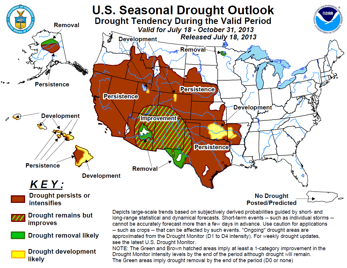
The Governor of Texas has asked the denizens of the state to pray for rain. The state has not had serious rain for months, and the drought conditions have turned severe.

The current drought conditions in Texas.

Conditions are not anticipated to get any better in the next few months. The recent predictions are that the conditions will persist in the area through July.

Predictions of the weather changes through July (NOAA )

Droughts around the world are one of the unfortunate consequences of changing weather, in much the same way as we have seen high snowfalls in other parts of the country this past winter. There will likely be cries about the underlying causes (with folks forgetting that droughts have occurred throughout history), but this post was started because of a potential event-changing occurrence.

This week Thames Water, which supplies 687 million gallons of water a day to the inhabitants of London and the immediate vicinity, was running its first water desalination plant. The region has faced droughts in the recent past as have other regions of the United Kingdom. Earlier solutions included building large water reservoirs, that at Kielder is the largest man-made reservoir in Europe. There is, however, only a certain limited amount of land that can be made available for this use, and so desalination proves an alternate way of supplying the increasing global demand for water.

In the United States droughts have threatened the viability of nuclear power stations, since the shortage of cooling water (as we recently learned again in Japan) is essential to safe plant operation. And therein lies one of the rubs to the situation. As the spokesman for Thames Water noted, the intent is not just to run the plant when there is a drought, since that is going to be too late. Rather at times of lower rainfall the plant (which can produce up to 150 million gallons a day) will pump clean water into the reservoirs, maintaining their integrity, and building up a reserve that will reduce the drought impact if it occurs. The plant was apparently completed last June at which time it was expected that it would just be used in times of drought. Within the last year that thinking has changed, and the plant is now running intermittently, partly to train operational staff, partly potentially also to help meet demand.

According to the Environment Agency, average water use is 148L per person per day in the UK and in the south-east of England it’s as high as 170L (far higher than the government target of 130L). Despite the popular perception of London as an overcast, rain-soaked city, its rainfall rate is, in fact, on a par with Rome, Dallas and Istanbul.

Schematic of the flow path through the desalination plant.

One question that I had relates to the amount of power that will be needed at Beckton. A calculation assuming that it takes 4 kWh to produce a cubic meter of fresh water, suggests that it will need a 21 MW plant. In 2009 the company CEO noted

The (20 MW) plant will be the first in the world to generate all its energy on-site, from renewable sources, including recycled cooking oil.

However the plant has been controversial, not least because although planning to use rapeseed oil, it could also burn palm oil, which is apparently cheaper. That is much more controversial. Planning permission for a second plant nearby at Southall, was refused in June 2010.

Biofuel powered stations in the UK, which includes that in the Tees Valley, where a plant burning 300,000 tons of recycled wood and specially grown wood from plantations, have had a somewhat mixed reception.

But to get back to the original idea of desalination, the largest plant in the United States is in Tampa with a maximum projected size of 35 million gallons/day, though it currently only produces some 25 million, sufficient for 10% of the region’s water needs. It went on line in 2008.

The plant uses about 44 million gallons per day (mgd) of seawater from a nearby power plant’s cooling system, which is pretreated with sand filters and a diatomaceous earth filtration system to remove particles. Reverse osmosis filters then separate 25 mgd of freshwater from the seawater. The unused concentrated seawater is diluted with up to 1.4 billion gallons of cooling water before it is discharged to the bay and that dilution is why environmental studies show no measurable salinity change in Tampa Bay related to plant production.

Which brings us back to Texas. In the latest report on desalination in the state, two possible developments are cited. There is a plan to install a 2.5 million gallon a day plant at Brownsville and a 1 million gallon a day facility on South Padre Island. Unfortunately the South Padre Island initiative failed in a bond election last year, and its future is considered doubtful. Meanwhile the Brownsville Public Utilities Board is considering combining a renewable energy source (shades of the UK) into the plant, in order to leverage funding, and possibly qualify for DOE funds.

But in the meantime, as the discussion continues, the drought gets worse. The discussions started with an initiative in 2002. As those in Texas may find out the hard way, waiting until the crisis is upon them makes it too late to construct the solution that might have helped. It appears that those in the UK and Florida were just a little more prescient. It might be noted that the initial planning for the Florida plant started in 1996.

Texas combined temperatures

This is one of an evolving series in which I am looking at the temperatures over the past 115 years in the different states of America. I started in Missouri, and have gradually changed the format of the post as I have found different things in my exploration of the data. Last week in looking at Oklahoma I changed the plot which compares the population around the measuring station to compare it with only the average of the last 30-years of temperature data, rather than the entire 115 years. This does not mean that the last 115 years of data is not valuable, though once I started collecting the GISS records for the state, I found that longer term range does not appear to concern them as much. Of the thirteen GISS stations listed for Texas, there are only three with a temperature record over the full 115 years. The remaining ten stations only have records since 1948.

There are 49 USHCN stations in Texas, ranging from Albany to Weatherford, and they are spread not quite evenly over the state.

Distribution of USHCN stations over Texas (USHCN )

Looking for the GISS station record for Austin I found that there are 3 different records in the GISS file the longest one, however, (1895 to 2009) is for an Austin at a different set of co-ordinates (39.5 N, 117.1 W) to the city which is the logical choice. Of course the currently used site (Austin/Robert 30.3 N 97.7 W) only has data from 1948, but then, so do the others I mentioned. Houston, for example, has four stations, but the one that GISS has chosen to keep maintaining records for has only been around since 1948. While it may be that I am more cynical than most it should be noted that, if one looks at the record for, for example, the GISS stations in Abilene and Amarillo, there are very clear higher temperature spikes in 1933 and 1934, above the most recent high temperatures.

Abilene TX temperatures (GISS)

Amarillo temperatures over the last century (GISS)

However if one only plots the temperatures since 1948 (as most GISS stations do) then there is no evidence that the temperatures were, in that record, higher than the recent past. For example consider the case of Lubbock as an example.

Historic temperature record for Lubbock TX (GISS)

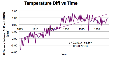
Looking at the overall temperature differences between the GISS temperature average, and that of the homogenized USHCN temperatures, there is a clear trend, although heavily influenced by the changing number of stations in 1948.

Difference between the average GISS station temperature and that of the homogenized data from the USHCN stations.

For Texas as a whole, of the average of the temperatures measured, adjusted for time of observation only (the TOBS temperatures) are used, then the state temperature appears to have declined slightly over the past 115 years.

Average temperature in Texas from 1895.

Texas is 790 miles long and 660 miles wide, including the bit that sticks up almost to Kansas and down past parts of Mexico. Thus it extends from 93.5 deg W to 106.5 deg W, and from 25.2 degrees N to 36.5 degrees N. is the second largest state, behind only Alaska in size. The mean elevation of the state is 518 m, and it runs from sea-level up to 2,666 m (Guadalupe Park). The average USHCN station is at a height of 438 m, while the average GISS station is at a height of 375.9 m. The Center of the state by latitude is sensibly at 31.25 degrees N. (both GISS and USHCN stations center on 31.3 degrees).

Turning to the usual geographic parameters, first latitude:

Correlation of temperature with latitude for Texas

Temperature correlation with longitude for Texas

However as the land rises to the West, this is explained within the relation to elevation:

Texas correlation with elevation

Using the 30-year temperature average for each station and plotting this against population, does not, for this state, give much of a correlation in this case

.Texas correlation of the last 30-year average temperature with population

And then there is the usual:

Difference between the reported USHCN homogenized data for Texas and the raw data corrected for time of observation (TOBS).

Sorry this is a little rushed today but a little excitement in the hotel with a fire alarm bringing us all down to the lobby and slowing things related to leaving. Nothing relative to the disasters of the rest of the world, but taking time.

It appears we can still have bad winters, right Texas?

The “historic” winter storm that is now heading East and then out of the country has had some significant effects, beyond just forcing folk like us out to shovel our driveways clear. Utilities in Texas were forced to impose rolling blackouts because of the shut-down of some of its generating power. This affected as many as 1 million homes. The problem was caused, in part, by broken and frozen pipes which shut off cooling water, and thus operation, at one coal-fired and one natural gas-fired electricity generating plant in the state. (SInce it "never gets that cold" in the state, the pipes were routed outside and installed without adequate insulation for the current weather, apparently.) At the same time, however, the exceptionally cold weather was causing a reduced flow of natural gas from local sources, so that backup power could not be brought on line.

Dewhurst said he was told that water pipes at two plants, one of which is Oak Grove , forced them to cut electricity production. Natural gas power plants that should have provided back up had difficulty starting due to low pressure in the supply lines, also caused by the cold weather.

(The other plant was Sand Hill).

While the system could normally buy enough compensating power from adjacent states, the large size of the storm system means that the power from those states was already being used, and even though spot prices rocketed (from $50 to $3,000 per megawatthour it was not enough to meet demand, and thus the power companies first imposed load shedding requirements, and then started the rolling blackouts. They have, at least for now, served their purpose, and ERCOT is reported as having ended them, at least for today. There remains a “strong possibility” that they will be re-imposed on Thursday.

Oh, and a minor comment, I was complaining to the Engineer (who is in Mass) about our weather and he laughed. He lives on the main street in Somerville, and they have had so much snow already that he doesn’t know where there is room to put what fell today, and which he has to move to get to his car. So far they have had, apparently, twice the amount of snow they get in a normal winter.

Climate scientists appear to have become so fixated on the likelihood of a continuing warming trend, and all the possible disasters that this might bring, that they leave Governments unprepared for any possible alternatives. Thus grit supplies were not increased this winter in either the UK or USA, dam levels were kept full in Australia, so that when a flood came there was nowhere to put the water, except down river – thus negating one of the very reasons the dams were put there in the first place. If it is not now apparent that colder weather can be at least as damaging as warmer, if not worse, then observational science, which used to have a considerable worth, has now yielded place to science by computer model, where the old GIGO rubric has been forgotten.

And if this post seems more like a rant, perhaps it is to do with the 3 hours it took to dig out my drive today, and the aches and pains that this has left in the aging corpus.

Problems for the Pickens' Plan

It is a relatively cool, overcast day here in Cambridge, MA, a little damp and after yesterday being chased up the New York Thruway by a storm carrying hail and cutting visibility to yards, (and the Fusion getting 41.6 mpg), only the occasional tree moved in an almost still day. Which is to suggest that it is not a good day for the prime candidates promoted as the sustainable fuels of tomorrow, here in the North East. That does not stop the tourists, however, and I noted as we came back to the hotel earlier this evening, that it was full and turning folk away. (Though it was easier for us to get rooms this year than last, and it is now offering a premium for those that stay over a weekend, and is giving away Internet services, neither of which held true last year).

The larger blow to the sustainable energy story today, however, is not the chill of an autumn day in July in Massachusetts, but rather the colder stillness of the lack of movement by Boone Pickens on his wind farm in Texas. The reasons for the turn around depend on who you read. The Wall Street Journal notes

Mr. Pickens, who has spent the last year pushing his "Pickens Plan" to reduce the nation's dependence on foreign oil, said the wind farm project was scuttled in part because of the lack of adequate transmission lines to carry the electricity from remote locations to cities. He had hoped to build new transmission lines but ultimately was unable to secure financing.

while Daily Finance noted the problems of raising money

Pickens, 81, was undaunted declaring at press conference on Capitol Hill, "I didn't cancel it ...Financing is tough right now and so it's going to be delayed a year or two."

"Cancel" may not be the right word. How about review? Pickens, who gained fame as a corporate raider in the 1980s, was planning to build the world's largest wind facility, at a site in the windy, flatlands near Pampa, Texas, which would generate enough electricity to power about 1.2 million homes.

The initial problem that Mr Pickens faces is that he has ordered the turbines and “like I said, my garage won't hold them," the legendary Texas oilman said. "They've got to go someplace."

There are 687 turbines involved, each to produce 1.5 MW of power and the question of where to put them, given that there are problems with the initial siting due to the need for connection to the grid, is likely to be a challenge. The problems have been visible for some time. Back in November there were signs that the credit crunch was hurting the program, and the drop in natural gas prices (which were the other half of the coin) has meant that there is no rationale for changing from natural gas to wind at the present time.

On the other hand, back this time last year the Texas legislature approved putting in the connections to bring the wind power into the grid.

Texas regulators have approved a $4.93 billion wind-power transmission project, providing a major lift to the development of wind energy in the state.

The planned web of transmission lines will carry electricity from remote western parts of the state to major population centers like Dallas, Houston, Austin and San Antonio. The lines can handle 18,500 megawatts of power, enough for 3.7 million homes on a hot day when air-conditioners are running.

The project will ease a bottleneck that has become a major obstacle to development of the wind-rich Texas Panhandle and other areas suitable for wind generation.

The transmission lines are needed since, at present, there is more capacity than can be delivered through the existing grid.

"When the amount of generation exceeds the export capacity, you have to start turning off wind generators" to keep things in balance, said Hunter Armistead, head of the renewable energy division in North America at Babcock & Brown, a large wind developer and transmission provider. "We've reached that point in West Texas."

Unfortunately that plan, shortly thereafter, ran into the Justice Department. The initial idea had been to integrate a water pipeline into the right-of-way so that Mr Pickens could also pipe water to Dallas and the water-short folk in East Texas from his holdings in West Texas.

At the time, Mesa General Counsel Bobby Stillwell said the company "got too clever."

Said Stillwell: "We had thought that doing them jointly would be a convenience and maybe even a cost savings to us and the landowners. There were two things that we misjudged. To do that we would have to acquire a 250-foot right of way instead of just a 150-foot one for electricity. That was enough difference to the landowners," he said. "Secondly, they were criticizing the whole project, both water and electricity, when they were really concerned about water. We didn't want both to be subject to the same criticism."

And so, last September, the water pipeline idea was scrapped, then the plan to use the wind power to displace natural gas was also put aside, and now the idea of the large wind farm itself has had to be laid aside.
But

Pickens continues to buy up water rights and says he expects to build smaller wind farms in Texas, as well as in Oklahoma, Kansas, and Wisconsin. He's still hopeful about his hedge funds, too.

This is occurring just as the President is sending out a team to encourage rural America to become involved in sustainable energy. It is not the best juxtaposition of events to see the sales pitch for wind included in their statements.

Wind energy offers rural landowners a new cash crop. Although leasing arrangements vary widely, royalties are typically around $2,000 per year for a 750-kilowatt wind turbine or 2% to 3% of the project's gross revenues. Given typical wind turbine spacing requirements, a 250-acre farm could increase annual farm income by $14,000 per year, or more than $55 per acre. In a good year, that same plot of land might yield $90 worth of corn, $40 worth of wheat, and $5 worth of beef." (Original Blogger's note: This report and its numbers are 5 years old. I've heard of lease payments of $5,000 per turbine.)

So just as I thought that wind was taking the commanding lead in the alternate energy stakes, we have days like today. Such events are bound to slow the growth of alternative fuels to the fossil fuels we now use, which makes the ongoing concern about the long-term viability of supply of those fuels ( worrisomely summarized by Sam Foucher at TOD) that much grimmer news.
.