Sunday, December 22, 2013

Tech Talk - The ExxonMobil 2014 Outlook for Energy

Each year the large oil companies produce their forecasts for future demand and supply of fuel, and these can be compared – both with earlier forecasts and with each other and the forecasts from different agencies. Last week, for example, I looked at the IEA forecast through 2035, while today’s subject is the ExxonMobil (EM) 2014 Outlook for Energy. (See also the 2013 Outlook Review and the 2011 Outlook Review).

In conformity with the IEA review EM consider that the energy growth rate for India will be perhaps one of the more significant metrics of the future. EM note that by 2040 one third of the global population will live in either India or China and between them they amount for half the global increase in energy demand, which is anticipated to be about 35% higher than the 2010 figure. India has already become the third largest energy consumer (after China and the United States).

One of the greatest drivers to energy demand growth comes as the population moves from the farms to the city and, as EM note, China has seen the urban population grow from 25 to 50% of the total in the past 20 years increasing residential power demand 20-fold. But that growth will slow in the future, reaching 75% by 2040. India (and Africa) are however further behind this curve with India being at 30% and Africa at 40%. Thus, as they still have further to move up the ladder, EM anticipate there will be concomitant increases in demand as these changes occur.


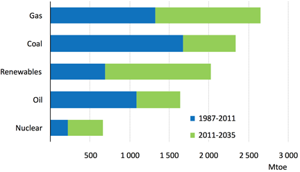
Figure 1. Projected growth in energy demand for major groups until 2040. (Illustrations are taken from EM The Outlook for Energy:A View to 2040 except where stated) (The key growth countries are Brazil, Indonesia, Saudi Arabia, Iran, South Africa, Nigeria, Thailand, Egypt Mexico and Turkey).

One of the small niggles with this projection is that it assumes a virtually limitless source of fuel.
Ongoing advances in exploration and production technology continue to expand the size of the world’s recoverable crude and condensate resources. Despite rising liquids production, we estimate that by 2040, about 65 percent of the world’s recoverable crude and condensate resource base will have yet to be produced.
While that projection will be discussed a little further later, it should be noted that in the next decade China’s energy demand will continue to grow at roughly current rates and that they have been quite assiduous in finding new sources to provide that energy. This is already providing some of the backstory to the growing tensions between China and its neighbors in the South and East China seas.

This is noteworthy because, as yet there is not much gap in the world between the quantities of fuels desired, and those available. Yet China is moving aggressively to ensure that it will be able to get what it needs when this changes. Such is not the case either with India, which has often failed in head-to-head bids for energy supplies when going against China, or much of the rest of the world who continue to accept the assurances that EM inter alia are promulgating with reports such as this, that there is a plentiful sufficiency.

Continuing along this unrestricted “ideal world” trail that EM are laying out, they continue to foresee that there will be a substantial improvement in energy efficiency over the next decades, leading to an increased decoupling of the relationship between GDP growth and Energy demand.


Figure 2. Projected growth in GDP and Energy demand through 2040.

Some of this EM project will come from the increased efficiency of automobiles and the greater acceptance of hybrid vehicles, with a penetration of 35% of the market – up from the 1% it held in 2010. While they do not expect that natural gas will have much impact on personal vehicles they do expect some impact with commercial transportation. The changes will lift the light vehicle mileage from the 24 mpg of 2010 to 46 mpg by 2040. (This is 1 mpg lower than their projection for mileage change given last year).


Figure 3. Changes in the composition and size of the global car fleet.

In terms of electricity supply EM foresee a sharply changing picture of the composition of the fuel sources for global supply, with coal barely holding its own throughout the period, and oil declining, while the remaining sources all grow in market size.


Figure 4. Sources of fuel and market size for electric power generation through 2040.

So where will the oil supply come from? Well EM remain confident in the future growth of North American oil.
North American liquids production is expected to rise by more than 40 percent from 2010 to 2040, boosted by gains in oil sands, tight oil and NGLs. With production rising and demand falling, North America is expected to shift from a significant crude oil importer to a fairly balanced position by 2030.

Latin American liquids production will nearly double through 2040 with the development of the Venezuelan oil sands, Brazilian deepwater and biofuels.

The Middle East is expected to have the largest absolute growth in liquids production over the Outlook period — an increase of more than 35 percent. This increase will be due to conventional oil developments in Iraq, as well as growth in NGLs and rising production of tight oil toward the latter half of the Outlook period.
The concern with these projections (which are substantially more optimistic than the IEA forecast, lies in their assumption of unfettered growth. As Ron Patterson just noted the EIA is anticipating that US volumes will peak in 2019, and then decline.


Figure 5. EIA projections for US petroleum production through 2040 (EIA).

Ron, has refined this plot and shows that US production may well peak in either 2015 or 2016, and go into significant decline by 2020. This is quite a contrast to the EM projection.


Figure 6. EM projection for change in liquids production through 2040

EM expect that Deepwater production will increase with major supplies coming from Angola, Nigeria, the Gulf of Mexico and Brazil, with production rising to a peak in around 2040. They expect tight oil supplies, however, to increase by a factor of tenfold from 2010 to 2040. The major new player in that field is anticipated to be Russia whose output is still expected to trail that in North America (which includes Canada and Mexico).

One of the great questions of the next decade relates to the development of the heavy oils of Venezuela and Canada. EM expects that the Canadian production will increase 200% with the rest of the total gain of 300% of the 2010 total presumably coming from Venezuela. However Venezuelan development remains a complex situation.

One of the most promising developments that EM describe is the use of extended reach horizontal wells, that are now allowing sub-sea deposits to be tapped using land-based rigs. At Sakhalin Island, for example, they note that they were able to drill one well in the Chayvo field that extended out 7 miles.


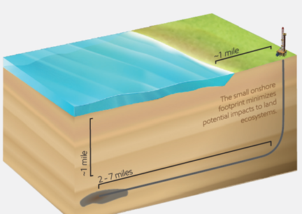
Figure 7. Illustration by EM of their extended reach well capabilities.

The other source that EM cite for increased production comes from OPEC and production gains in the Middle East. Given that Saudi Arabia have stated that 10 mbd is their intended upper limit to production (give or take a little) one presumes that the roughly 9 mbd gain is largely anticipated to come from Iraq. EM don’t actually say, nor did they last year, but it is interesting to end by comparing last year’s projection for future growth with the one shown in Figure 6.


Figure 8. The projected volumes for liquid supply growth as provided by ExxonMobil last year in their 2013 report.

On which cheerful note I wish you all the Compliments of the Season, and hopes that you have a safe and happy break.

Read more!

Wednesday, December 18, 2013

Waterjetting 16c - Optimal AFR and cutting curves

The discussion on surface quality which forms this month’s topic has, to date, focused on linear cutting since this has been the simplest way of explaining some of the factors that go into choosing an optimum abrasive feed rate (AFR) for a system. Along the way, however, I have pointed out that the internal design of an abrasive nozzle has a considerable impact on the relative performance of different systems.

If, for example, the internal geometry is such that there is not an optimal transition of energy between the high-pressure waterjet stream and the abrasive particles, then trying to draw conclusions over the influence of some of the operational parameters, such as pressure, can lead to false conclusions. The optimal AFR changes with the relative sizes of the waterjet orifice, the location of the abrasive feed line, the length of the mixing chamber and the geometry of the focusing tube. These parameters are generally held fixed since most folk buy only one cutting head design, and tend to stick with it once purchased. However, as I pointed out at the beginning of this blog, there is a considerable difference between the performance of different abrasive cutting heads.


Figure 1. Comparison of the relative cutting performance of twelve different abrasive nozzle designs, when operated otherwise at the same pressures, water flow rates and AFR.

The best design, for the particular waterjet and AFR parameters that were tested in generating Figure 1, was 24% more effective than the average performance of the nozzle designs tested. This is indicative that the design was more efficient in accelerating the abrasive to a higher velocity than the competing designs. Those designs were tested at a number of pressures and AFR values to ensure that the conclusions held within the range of test – and they did. But as the pressures and AFR values change so there is a change in the optimal design with consequences on the optimal AFR as it relates to the operating pressure of the system.

Without an awareness of these inter-related parameters it is possible to draw erroneous conclusions about the best choice of cutting parameters for a given operation. The situation becomes even more complex where the paths being cut are no longer straight but involve complex contour cutting, and where there are requirements for zero taper and high surface quality on the cut faces of the part being generated.

One solution to the problem is to accept the limitations of the system, and cut the part at a constant speed, slow enough that the jet cuts through the piece on first contact with the abrasive stream over the length of the cut. (In other words after the abrasive bounces away from the initial contact plane along the cut it does not meet any more material before it exits from the bottom of the cut). At a pressure of 40,000 psi the cutting speed to achieve these requirements over an half-inch thick titanium target lies at around 0.3 inches per minute.


Figure 2. Change in cut face taper angle with traverse speed at a cutting pressure of 40,000 psi.

However as the pressure of the jet is increased the cutting speed to sustain that quality cut goes up significantly, so that there is a significant benefit to the increased pressure. But the optimization to achieve this is geared to ensuring that the optimal abrasive feed rate has been selected, for a given nozzle design and waterjet pressures. Without a short series of tests to ensure that the system is being run at this optimal condition it is not possible to accurately state how a system can best be used.

I have described, in an earlier post, how such a simple test can be run. It should be stressed, however, that the selection of an optimal AFR for a nozzle is based on the nozzle geometry and the operating pressure of the system. That selection will provide the best cutting jet and this jet will have different capabilities in different target materials. Composite materials will cut at a different optimal speed depending on the material type and thickness, and these values will differ when metals, or ceramic materials are being cut. But, as a general rule, the selection of the best cutting conditions are first established by knowing the thickness and type of material to be cut. This should then produce, based on tested performance tables, recommendations for the cutting speeds at different pressures, where the cutting pressure in turn defines the optimal abrasive feed rate. Based on an assessment of the different categories of cost of an individual operation one can then decide which set of conditions would provide the most economical and acceptable answer to providing the quality of cut required.

In some cases it may be that the cutting head can be tilted so that, particularly with straight cuts, the part being isolated will have a perpendicular edge, while the scrap piece will have a tapered edge at twice the normal angle. For example under the conditions illustrated in figure 2 tilting the nozzle by only one degree will allow cutting at 4 ipm rather than 0.3 ipm, a 12-fold gain in performance, depending on the assurance of the quality of the surface being sustained.

As mentioned earlier this option becomes more difficult as the part being cut acquires contours. At higher pressures the angle of the cutting face curve is reduced, but in thicker parts there is often a slight displacement backwards (a rooster tail as it is sometimes called) from the top edge of the cut to the bottom. When the nozzle comes to cutting around a curve that backward projection at the bottom of the cut can pull the cut edge away from vertical unless the cutting head is adjusted to ensure that this difference is minimized to the levels acceptable to the customer. Most commonly this is achieved by slowing the head speed according to the radius of the curve, with sharper turns being made at slower speeds. Some adjustment in the angle of the head can also be made, but this requires a more advanced method of control and programming in developing the cutting path for the head.

Note: Because of the season this site will be Dark next week, so let me take the opportunity of wishes the readers of the waterjetting series all the Compliments of the Season, and with hopes that you have a Prosperous and Happy New Year.

Read more!

Tuesday, December 17, 2013

Tech Talk - The IEA World Energy Outlook

It is the time of year again that different folk stare into their own versions of a crystal ball and project how much energy the world will need in the future, and where they think that it will come from. It is interesting to look at these various predictions as the global supply picture morphs under a changing reality.

One of the changes in reality that is likely to have significant impact in the near-term is the flow in the Alyeska pipeline. Long-time concerns over the decline in flow and the effect that heat loss has on the contents is leading to new work to change the pipe dynamics and possibly to remove the water before it is pumped, lowering the temperatures at which the line currently has to be maintained.


Figure 1. Historic and Projected flows through the Alaskan pipeline (Alyseka)

The precipitation of ice and water from the oil, within the pipeline will otherwise reach a point that flow will stop – potentially at around 300 kbd, at a date not too far into the future.

In their annual World Energy Outlook, the IEA continue to see, overall, a gain in US oil production through 2025, largely coming through the light tight oil of the sort being produced from North Dakota and West Texas.


Figure 2. IEA projections for global oil production growth in the years to 2035. (IEA)

However in the following years , out to 2035, that supply also declines so that by 2035 the US will likely be in the same sort of supply situation, relying heavily on imports, that it is today.

The IEA make the point that the only longer term places that can be relied on are Brazil, with the off-shore fields, and the Middle East. Looking first at Brazil, which continues to have some problems in bringing their fields on-line on-schedule, the IEA anticipates that the major production growth is likely to be in the next ten years, but will continue beyond that point.


Figure 3. Brazilian oil production through 2035. (IEA)

Because the IEA foresee that Brazil will continue to supply the largest portion of its energy from hydropower this means that the largest volume of the fuel can be exported, where it meets the continually growing demand from the rest of the world.


Figure 4. Anticipates sources of power for electricity generation in 2035 (IEA)

At the same time the IEA anticipate that primary energy demand will still focus heavily on fossil fuel sources through 2035, with renewable energy only slowly nibbling away at the totals so that, by 2035 fossil fuel will have dropped from contributing the current 82% down to 75% of the larger total.


Figure 5. Anticipated changes in the sources of primary global energy through 2035. (IEA)

Although, by that time the IEA foresee a change not only in the places where demand is highest, but also in the relative rankings. The major finding in this regard that they draw attention to is the anticipated greater growth rates in India than in China, as time passes.


Figure 6. Changed picture of global energy demand in the year 2035 (IEA)

Other than projecting the growth in demand there is the need to anticipate where the supply will come from, and in this regard the IEA projects that the largest growth will come from natural gas (Figure 5), although crude oil is still anticipated to grow, with refinery capacity increasing to about 104 mbd.

It is interesting that the IEA projections for oil production growth hang most heavily on increased production from the Middle East. It requires very little glance into their crystal ball to assume that this is likely based on the increased production from Iraq, an assumption that was, last year, a largely common assumption to all future projections. Unfortunately for those earlier projections in the interim the initial Iraqi targets have been cut back, with current targets being reduced below the “best case” scenario that the IEA had projected in their review of the country.

Taken with the possibility of a significant and sudden decline in production from Alaska, and the likelihood that the rate of drilling in the Bakken will decline, as prospects become more uneconomic suggests that it will be difficult to sustain the levels of crude output that the IEA are anticipating can be made available to meet their projected needs.

By the same token the growth in the global demand for natural gas is predicated on the reserves uncovered in the United States being exported, as needed, to the rest of the world. It is, however, also predicated on the price of natural gas remaining relatively stable in terms of current costs.


Figure 7. Anticipated components of the costs of US LNG when shipped to either Asia or Europe (IEA)

The underlying flaw in that assumption is that the costs of purchasing the natural gas in the United States are now starting to rise to a more realistic level relative to the costs of production from tight shales. This week's OGJ, for example has noted the EIA Short Term Energy and Winter Fuels outlook that notes that prices are expected to rise 13% this winter over last (on constant demand) to $3.62 per kcf. Given that the EIA is expecting the price to inch upwards towards $5.00 per kcf over the next year this makes the IEA report appear a little over-optimistic on costs and hence market share.


Figure 8. Natural Gas Prices in the United States (EIA)

This is likely to be particularly true as some of the older gas fields, such as the Haynesville, appear to be in decline even at prices in the $4 - $5 per kcf range.


Figure 9. Natural Gas Production from the Haynesville Shale (OGJ )

Increasing the price of natural gas will reduce its competitive advantage over coal and in consequence I would anticipate that power generating companies will continue to build boilers that can handle both coal and natural gas, and that the longer-term continued switch to natural gas will become more of an economic choice dependent on how much LNG finally comes onto the market from the United States and at what price. I am not convinced that this will be quite the bargain and cornucopia that it is anticipated to become. In other words I still find the IEA view of the future to be a somewhat optimistic one, given the realities that are now unfolding before us.

Read more!

Tuesday, December 10, 2013

Waterjetting 16b - Optimum Abrasive Feed Rate and Depth

The post that I wrote last week was focused on the misperception that you need to add more abrasive to an abrasive waterjet if you wish to cut through thicker material. This is wrong on a number of counts, but most particularly because a good operator will have tuned the nozzle to achieve the best cutting jet, based on pressure and abrasive feed rate (AFR) regardless of target material. What the operator may change is the operating pressure (which would change the optimum AFR) and the traverse speed since these control the depth and quality of the cut that the jet makes.

But, before leaving the topic, I would like to discuss, in a little more detail, the concept of the optimal amount of abrasive that one should use with a given jet, and what happens as that feed rate is changed. As I mentioned last time, because of differences in the shapes of the mixing chambers of the nozzles supplied by different manufacturers, the specific sizes and optimal flow rates will differ from nozzle to nozzle but the overall conclusions remain the same.

Last time I pointed out that the driving waterjet had to break up within the mixing chamber in order to properly mix with the abrasive and to bring this up to a maximum speed before the mix left the focusing tube. Where the driving jet is too large then this breakup is not complete and the mixing is not efficient. As a result the jet that comes out of the end is more diffuse and the abrasive will not have reached the full velocity possible. However, if the incoming waterjet is made smaller for the same AFR and other mixing chamber geometries, then the cutting performance will decline.


Figure 1. Effect of increase in jet pressure when cutting aluminum with an AFR of 1.7 lb/minute (after Hashish, M., "Abrasive Jets," Section 4, in Fluid Jet Technology- Fundamentals and Applications, Waterjet Technology Association, St. Louis, MO, 1991.)

For a similar reason adding a polymer to the jet fluid should only be carried out with some care for the consequences. Long-chain polymers can give a jet increased cohesion and this can, at high enough concentrations, inhibit jet breakup in the mixing chamber thus reducing the effectiveness of mixing in the chamber.


Figure 2. The effect of changing cutting fluid on AWJ performance (after Dr Hashish ibid)

Polyox, (polyethylene oxide) is an extremely effective polymer for increasing jet performance by cohering the jet and reducing the friction losses between the pump and the nozzle. However, as the graph shows, adding it to some abrasive systems will reduce performance since the more coherent jet makes it more difficult for the abrasive to mix and accelerate to full velocity. At lower concentrations the polymer allows the jet to breakup, but keeps the slugs of water together making energy transfer more efficient. Higher velocity abrasive means that less is required to achieve the same cutting performance as Walters and Saunders showed.


Figure 3. Effect of adding polymer in reducing the amount of abrasive required to cut stainless steel (after Walters, C.L., Saunders, D.H., "DIAJET Cutting for Nuclear Decommissioning," Paper J2, 10th International Symposium on Jet Cutting Technology, Amsterdam, Netherlands, October, 1990, pp. 427 - 440.)

At low levels of abrasive feed Dr Hashish has shown that increasing the amount of abrasive in the feed increases cutting performance.


Figure 4. Effect of increase in AFR on depth of cut in mild steel at a feed rate of 6 inches/min (After Dr. Hashish ibid), waterjet diameter 0.01 inches.

However, as the abrasive flow rate continues to increase the cutting performance reaches a plateau and can decline, as Dr. Hashish illustrated. An AFR of 20 gm/sec is equivalent to a feed of 2.6 lb/minute.


Figure 5. The effect of higher AFR on cutting depth at 3 jet pressures on a mild steel target (after Dr. Hashish ibid)

Note that in this case the nozzle geometry was not optimized for operation at the highest jet pressure. More visibly we ran a series of cuts across a granite sample, where the only thing that changed between cuts was that we increased the abrasive feed rate in cuts from the left to the right. It can be seen that beyond a certain AFR the jet starts to cut to a shallower depth.


Figure 6. Successive cuts made into a granite block at increasing AFR from the left to the right.

Interestingly the optimum feed rate doesn’t just depend on the pressure and water flow rate (waterjet orifice size) of the system. Faber and Oweinah have shown that as the feed particle size gets larger, so the optimum AFR reduces.


Figure 7. Optimal Abrasive feed rate as a function of particle size (after Faber, K., Oweinah, H., "Influence of Process Parameters on Blasting Performance with the Abrasive Jet," paper 25, 10th International Symposium on Jet Cutting Technology, Amsterdam, October, 1990, pp. 365 - 384.)

The process of finding an optimal feed rate for a system is thus controlled by the design of the mixing chamber based on the relative position of the abrasive feed tube and the size of the waterjet orifice. This controls how well the abrasive that is fed into the system can mix with the jet and acquire the velocity that it needs for most effective cutting. Then, as the above plot shows, the optimal AFR is also influenced by the size of the particles that are being fed into the system, since as the particles become larger beyond a certain size, so the cutting effectiveness declines.

Part of the reason for this is that, as the AFR increases so there is an increased risk of particle to particle impact breaking the particles down into smaller sizes. (And an earlier post showed that smaller particles cut less effectively – as does figure 7 above). We screened the particles that came from several different designs of AWJ nozzle assemblies capturing them after they left the nozzle but without further impact, so that the size range is indicative of that which a target material would see,

The table is a summary of some of the results and it shows results for a feed that began at 250 microns giving the percentage of the particles that survived at larger than 100 microns.


Figure 8. Percentage of the 250 micron sized feed that survives at above 100 micron for differing jet conditions. (the numbers are averaged from several tests).

It can be seen that when the feed rate rises to 1.5 lb a minute that there is a drop in abrasive size at higher jet pressures, and this is likely to be due to the increased interaction with particles. Since cutting effectiveness is controlled by particle size, count and velocity the only slightly greater amount of particles that survive above 100 microns at 1.5 lb/minute relative to those that survive at 1 lb/minute suggest that spending the money to increase the AFR above the optimal value (in this case around 1 lb/min) is a wasted investment.

It is therefore important to tune the system to ensure that, for each jet pressure and nozzle design that is used, that the AFR has been optimized.

Read more!

Tech Talk - a gentle cough for Simon Michaux

In response to a post I wrote a couple of weeks ago Marty suggested that I watch a video by Simon Michaux discussing peak mining. So I did.

A quick check through Linked In has Simon Michaux as a Mining Consultant in the Brisbane area, having been a Senior Research Fellow at the Julius Kruttschnitt Mineral Research Center (JKMRC) at the University of Queensland for 14 years. (I should mention I spent a sabbatical at the Mining Department at the University of Queensland in 1987).

In his presentation Simon discusses Sustainability in regard to the mining industry, pointing out that as the population rises and demand for minerals increases, that demand can only be met by mining leaner and deeper ores, once the shallow easy and cheap to mine deposits are gone. (A similar argument to that of peak oil, which he does talk about in his presentation as well as mentioning the predictions that we are nearly at Peak Coal).

I have a number of problems with his approach, and have discussed some of them in various posts over the past few years, but let me discuss them again as a rebuttal to his conclusion that the world is rapidly heading into disaster and the end of the Industrial Age as the costs to mine minerals and the difficulties in finding enough product make it impossible to continue our current trends.

Now it is true that back in the days when Europeans first came to the United States that the local tribes around the Great Lakes were mining pure copper strips and large slabs and nuggets could be found. White Pine Copper Mine in Michigan was still finding these when I visited there some decades ago, but they occurred in a relatively hard host rock and the deposit was going deeper and becoming more expensive and so the mine closed. Because of economies of scale it became cheaper to simply dig much lower grade ores out of the ground. He cites the example of Bingham Canyon where the mine now extracts copper from ores with less than 1% of disseminated copper, rather than the pure copper nuggets of former times. And he points out that as the ore is ground finer it requires more power.


Figure 1. Relationship between energy required to liberate minerals from ore by reducing the particle size, leading to higher energy demands. (Simon Michaux)

There are a couple of points that need to be raised here. The first is that digging ore (and coal) out of a surface mine is a relatively simple and comparatively inexpensive operation. It does not require large applications of exotic technology and the whole process of getting the ore from the solid to the point where the mineral is liberated is straightforward.

The reason that there are steel balls shown on the rhs of the above figure is that after the body of the ore is broken free with explosives the fragments are picked up in a large shovel and loaded into mine trucks that carry hundreds of tons at a time to the main plant where the ore is crushed in part by falling into long rotating drums filled with steel balls that break the rock into fine particles through impact and attrition. (A simplified modern version of pounding the rock fragments with hammers until it gets small enough to free the mineral). Simon makes the point that modern technology is now capable of breaking the ore down to 5 micron particle sizes to free the ore, but that this takes increasing amounts of energy (as shown above), and that hauling all the ore to the plant and crushing it all to this small particle size is leading to unsustainable energy costs – particularly as oil and other fuel prices are set to continuously rise in the future.

But here he makes a critical misjudgment, because his argument rests on the mining industry and the manufacturing industry remaining the same, and following conventional practices into the sunset. But this is unlikely to happen. Just as the increase in prices made it possible to develop hydrofracking of long horizontal wells and thereby develop the oil and gas in the otherwise uneconomic deposits of Dakota and Pennsylvania so technology can find alternate processes that will lower the costs for mining minerals.

For example it is not necessary that the trucks that haul the ore rely on diesel fuel produced from oilwells. Some mines have already switched to biodiesel, which has some advantageous properties for their operations. Other mines use electrical power to run their haulage and GE has demonstrated that diesel engines can run on a mixture of fine coal and water. The reason that countries such as the UK have migrated away from coal use has more to do with the availability of cheaper sources of alternate fuel and for political reasons rather than there being a lack of available coal. (Note that German use of coal for power is increasing as an example).

Secondly the use of ball mills for crushing all the ore is simple but not necessarily all that efficient. I have noted that a more efficient process, wherein ore can be reduced in one step from 1 cm size to 5 micron size, using cavitation, is quite easy to build and operate.

The use of hydroexcavation and instant ore comminution using cavitation means that the ore can be separated into mineral and waste at the mining machine, and (because of the way the process works) both fragments of the ore are broken at the natural grain size, so that there is no need for overgrinding, and the fragmentation is by tensile fracture growth instead of compressive crushing, saving energy. By separating the mineral at the face, and leaving the waste in larger fragment sizes the waste can be relocated close to the mining face, potentially being used to provide support in regions that have been mined out. Only the mineral needs to be moved from the face to the plant – cutting energy costs dramatically.

Once the mineral is available as a fine particle it becomes easier to treat it and process it into the required feedstock which, as 3D Printer technology migrates into the construction of larger and more useful items from metals and more advanced materials so the waste involved in older conventional practice will be minimized and costs in financial and material items contained.

The future is likely therefore to be much more exciting and positive than Simon Michaux foresees, though I do agree that it will become more sensible to mine landfills to reclaim minerals – but then we have been doing that for some time now. But no, we are not coming to the end of the Industrial Revolution, merely moving to a different phase.

Read more!

Friday, December 6, 2013

Waterjetting 16a - Abrasive Feed

I was talking with someone the other day who mentioned that it was necessary to increase the amount of abrasive feed to a waterjet whenever the material to be cut was thicker. This is actually a myth, or put another way, wrong! It is the equivalent of saying that you should use a duller knife if you want to cut thinner material.

Today’s topic therefore is about optimizing the abrasive feed rate into an abrasive waterjet cutting system, but you should remember that different manufacturers have different nozzle assembly designs. Thus the graphs and tables that I will use to illustrate the discussion relate to one particular nozzle design that was used at that time. Not all the nozzle designs were the same, but the results illustrate the points that I am going to make. But it underlies the recommendation that you should each run some standard tests with your system so that you have a baseline of performance and data to tell you where your system works best.

There are several reasons why different designs produce different cutting results, and I will point out some of them in what follows. To begin, however, consider again the basic elements of the waterjet mixing chamber.


Figure 1. Section through the mixing chamber of a conventional abrasive injection system.

A small high pressure stream of water enters the chamber through the upper nozzle, passes through the chamber, creating a vacuum that pulls abrasive into the chamber, and mixes with that abrasive before the resulting AWJ exits through the focusing tube.

One of the first things to understand is that, in the cutting jet that issues from the tube the actual cutting comes from the abrasive particles. From work that has been carried out at a number of places we know that the higher the velocity of the particles, the greater the damage that they will do on the target.


Figure 2. Relative mass loss when steel balls hit a mild steel plate (after Hutchings, I.M., Winter, R.E., Field, J.E., "Solid Particle Erosion of Metals;The Removal of Surface Material by Spherical Projectiles," Proceedings of the Royal Society, London, Vol. A348, 1976, pp. 379 - 392.)

Discussion in earlier posts pointed out that there are different ways in which waterjets attack ductile and brittle materials. However the relationship between an increase in impact velocity and damage occurs whether the targets are brittle or ductile. In figure 2 the target was a ductile steel, in more brittle material it is the coalescence of cracks that removes material, and higher velocities create larger cracks, as shown in figure 3.


Figure 3. Effect of impact velocity on crack length, (after Evans, A.G., "Impact Damage Mechanics: Solid Projectiles," in Erosion, Treatise on Materials Science and Technology, Vol. 16, ed C. Preece, Academic Press, 1979.).

And the same form holds true if steel balls are fired into sandstone.


Figure 4. Relative amount of Berea sandstone removed by the impact of steel balls of varying size (after Ripkin, J.F., Wetzel, J.M., A Study of the Fragmentation of Rock byImpingement with Water and Solid Impactors, Final Report on U.S. Bureau of Mines, Contract HO 210021, February, 1972.).

The above graphs show that it is more effective to have the abrasive moving faster in terms of the damage done by individual particles. Which brings up the first consideration in the design and use of an AWJ mixing chamber.

In order to get the particles moving as fast as possible they have to get their energy from the water jet entering the chamber. But the jet enters the chamber as a solid stream that then breaks into droplets (as shown in earlier pictures) as it passes down the chamber. If the jet remains in a solid stream all the way down, and out of the focusing tube, then the abrasive will find it difficult to penetrate into the center of the jet stream and pick up all the needed jet energy.

This can be illustrated by looking at the velocity and distribution of particles coming out of a nozzle with two different sizes of waterjet orifice but the same size of focusing tube diameter.


Figure 5. Relative particle distribution across a 40,000 psi jet with a focusing tube diameter of 2.3 mm (0.09 inches), and an AFR of 1 lb/min for two waterjet orifice sizes (after Mazurkiewicz, M., Olko, P., Jordan, R., "Abrasive Particle Distribution in a High Pressure Hydroabrasive Jet," International Water Jet Symposium, Beijing, China, September, 1987, pp. 4-1 - 4-10.)

The smaller waterjet breaks up fully within the chamber entraining and accelerating the abrasive particles and providing the desired cutting stream. The larger sized jet does not completely breakup, and fewer particles can mix into the center of the jet giving a more diffuse and less efficient cutting stream. In this case changing from a 0.005 inch waterjet orifice to a 0.013 inch diameter orifice (at roughly 7 times more power, because of the higher flow rate) produces a poorer result.

It is therefore important to ensure that there is an efficient energy transfer between the water and the particles. But the jet energy can only be diffused to a certain number of particles before it significantly begins to reduce in the amount of energy that it imparts to each particle. In other words if you put too much abrasive into the jet stream, then the amount of energy each particle gets is reduced, as it the overall cutting efficiency.

In an example I have used in class I noted that if I pick up a small child and run down the corridor, then I can carry the child at about my normal running speed, on the other hand if I pick up a couple of football players and try the same run I will be barely able to stagger. So the optimum carrying capacity of any jet can be determined for a given water flow rate, which is itself based on the waterjet orifice diameter and the pressure at which the water is supplied.

I will return to this topic next time, but you can see, in the concluding figure, that when a lower abrasive feed rate is fed to the nozzle, that the percentage of the abrasive moving in the higher velocity range rises to over 60% compared with only 20% of the particles when the abrasive feed is too high. And that means that the cutting performance will be less with the higher abrasive feed rates. (The numbers are a little high to reinforce the point).


Figure 7. Particle velocity distribution on leaving the focusing tube (after Isobe, T., Yoshida, H., Nishi, K., "Distribution of Abrasive Particles in Abrasive Water Jet and Acceleration Mechanism," paper E2, 9th International Symposium on Jet Cutting Technology, Sendai, Japan, Oct, 1988, pp. 217 - 238.)

Read more!

Tuesday, December 3, 2013

Tech Talk - Falling gas prices and Iraq

Filling up at the local gas station yesterday I noted that prices are still below $3.00 a gallon, though at $2.99 only just below. Going back to the BBC Calculator this is still $2.04 less per tank than the regional average, and $86 less than I would pay in Italy. So even though the costs are rising over the last time I looked, they are still relatively low.


Figure 1. Relative fuel costs ($/gal) in different locations around the world. (BBC Calculator)

The orange line in figure 1 shows what I paid, and the darker grey horizontal line the regional cost here in the MidWest.

The EIA have noted in last week’s TWIP that the national price is as low as it has been since the beginning of 2011.


Figure 2. Average US retail prices for gasoline (EIA).

The EIA continues to describe the causes of these relatively low prices:
Lower global crude oil prices, high profitability for diesel fuel that has been encouraging refiners to increase throughput, high inventories, and the switch to less-costly winter grades of gasoline are among the factors currently driving gasoline prices.
The OPEC Monthly Oil Market Report (MOMR) reports that global oil prices have fallen $2.04 a barrel (to $106.69) – the first decline in five months, as stocks increase and the Northern Hemisphere moves into winter. The estimate for global demand growth this year remains at 0.9 mbd, with the growth for next year anticipated to be at 1.04 mbd. This steady growth in global demand of a million barrels a day keeps raising the question as to where the increase is likely to come from. This is particularly germane given the disturbed conditions in a number of the MENA countries that provide a significant amount of baseline production, as well as anticipated increases.

The problems in Iraq, for example, have now reached the point that the Turkish government is directly working with the Kurds in Northern Iraq, to develop the oil in the Kurdish northern part of Iraq. This comes at a time that Iraq has been negotiating with the different major oil companies that had contracted to help Iraq reach an overall production target of 12 mbd by 2017. There have been considerable doubts cast on that original estimate, with the IEA producing a report, reviewed in an earlier post that concluded that the country would be lucky to achieve a production goal of 6 mbd by 2020, with an out year estimate that the country would be able to reach 8.3 mbd only by 2035.

Recognizing some of the difficulties in gearing up oil production at the different oilfields around Iraq (some of which were discussed in another post last June) production targets for 2017 had already been scaled back to a goal of 9 mbd by 2017, a drop of 25%. Now there has been discussion between Iraq and its partners for the various fields to drop those target values further, despite the large scale of the reserves that are considered available.


Figure 3. Oil reserves by field (Financial Times)

Exxon Mobil had 60% of the stake in the West Qurna oil field, but after it had started to work with the Kurds independently of Baghdad it found that relations with the Central Government rather chilled. Exxon Mobil has thus sold 25% of their stake to Petro China, and 10% to Pertamina of Indonesia, bringing the EM stake down to 25%. The current discussions between the companies and the Iraqi government are aimed at reducing the production target of the field by around 1 mbd..

Oil has just started to be produced at West Qurna Two, but the initial target is to have commercial production by the end of the year has suffered from local disruptions and the initial goal to reach a production of 400 kbd by the end of 2014 is now also in doubt. Commercial production is now not estimated to begin until perhaps the end of the first quarter of 2014. Initially the field was to be producing 1.9 mbd by 2017. That goal had been lowered to 1.2 mbd at the end of 2012. How the current disruptions will play into that target is difficult to estimate yet, but a year ago the parties were assuming that production would have already reached 150 kbd.

Earlier this year ENI had agreed with the Ministry of Oil to lower the target peak production from the Zubair field from 1.2 mbd to 850 kbd with that goal to be reached in 2016.

Discussions are not yet complete on new target production to be achieved from the Majnoon field. Shell has just announced the start of production from the field with the intent of raising production to over 175 kbd by the end of the year. However the long term target of raising production to 1.8 mbd is now in question. Shell is reportedly suggesting that the 2017 target be lowered to 1 mbd.

Similarly over at the Rumaila field BP is in discussion over long-term production, although earlier last month Schlumberger stopped work at the field because of local disturbances. With the field producing 1.4 mbd the disturbance was short-lived and is not reported to have affected current production, though it is indicative of tensions within the country. Current discussions are aimed at lowering the 2017 target production by around 800 kbd.

When these cuts are combined the total reduction is around 3.65 mbd, taking 2017 production down to 5.35 mbd, which is below the earlier best case scenario envisaged by the IEA.

OPEC notes that, after reaching a peak recent production of 3.194 mbd in August, production has fallen back below 3 mbd in September and October, and with Saudi Arabia also cutting back below 10 mbd in October the Organization is lowering production to meet the reduced winter demand, albeit the reduction from Iraq might not have been anticipated.


Figure 4. OPEC production figures through Oct 13, 2013 as reported by others to OPEC (OPEC MOMR )

This means, unfortunately, that if the world was anticipating that the roughly 4 mbd increase in global demand by 2017 would be met largely by increased oil production from Iraq then they are likely to be sadly disappointed. Enjoy the lower gas prices while you may.

Read more!

Sunday, December 1, 2013

Waterjetting 15d – More thoughts on cut surface quality.

When a high-pressure stream of water hits a surface, the arrival of subsequent lengths of the waterjet stream forces the initial water away from the initial impact point, into and along any weakness planes in the target material. As a result there is some preferential cutting of the material, especially where there are defined weakness planes in the material. One illustration of this is where a jet that contains cavitation bubbles impacts on a rock surface (figure 1) and as the water enters the narrow eroded channels where preceding lengths of water have preferentially eroded out the weaker rock the pressure in the channel increases, collapsing the remaining cavitation bubbles and further exacerbating the damage within that narrow channel, causing it (them) to grow preferentially relative to the surrounding rock.


Figure 1. Looking down into a channel cut by a cavitating jet that traversed from left to right, at a speed of 0.4 inches/minute. Note the preferential attack into weakness planes within the rock.

As the weakness planes grow and join, so individually larger pieces of rock can be broken free from the target and the path, and pressure profiles of the water in the cutting zone change quite significantly. For this cavitation to have a significant impact on the erosion pattern, however, the traverse speed over the surface must be controlled, and be relatively low. At more effective speeds the cutting process does not allow for the development of this fracture mechanism. Rather, with plain jets, the process concentrates just on crack growth around individual grains. Optimum cutting speeds are much higher, depending on the intended result.

The efficiency of waterjet cutting has, historically, been assessed in terms of how much energy is required to remove unit volume of material. This we call the specific energy of the cutting process, and a common unit is joules/cubic centimeter (j/cc). When using a waterjet to cut into material, in part because of the interference between different segments of the jet stream, pre and post impact, the most efficient cutting speeds are quite high.


Figure 2. The change in cutting efficiency with traverse speed of a high-pressure waterjet cutting stream

The downside to using higher cutting speeds (apart from the simple inertial problems in driving systems at higher speeds in other than straight lines) is that the depths of cut achieved become smaller on individual passes, as the jet has less cutting time on each path increment.


Figure 3. Change in cut depth as a function of traverse speed, for varying different rock types.

In linear cutting systems it is sometimes possible to align secondary or a higher multiple array of nozzles along the cut, so that thicker materials can be cut with a sequence of jet cuts along the same path. Alternately a single nozzle can make multiple passes along the cut path and sequentially deepen the slot.

Unfortunately while this is an effective way of solving some problems, it becomes less efficient as the slot gets deeper.


Figure 4. The change in cutting efficiency with increase in the number of cutting passes.

At higher pass numbers with the target surface at a growing distance from the nozzle, and with the edges of the cut starting to interfere with the free passage of the jet to the bottom of the cut, less energy is arriving at the bottom of the slot and thus the effectiveness falls.

While there are differences between abrasive waterjet cutting (where the optimal cutting speed is much lower than that for a plain high-pressure water jet) the form that the cutting jet takes through the target material is of similar shape in both circumstances.


Figure 5. An abrasive waterjet cut through 1-inch thick glass

As the jet cuts through the piece, so the cutting edge curves backwards from the top of the cut to the bottom. The rate of this curvature is, inter alia, a function of how fast the nozzle is moving over the surface. Dr. Ohlsson showed this effect in cutting through 0.4-inch thick aluminum and mild steel plates, back as part of his doctorate at Lulea in 1995.


Figure 6. Change in the cutting edge profiles and cut groove patterns in metals as a function of cutting speed (L. Ohlssson PhD Lulea, 1995)

The growth of the striations in the cut surface, as the depth of cut increases is one of the larger concerns with cut surface quality, since customers are often concerned that these be minimized, and further if they become large enough they can make it difficult to separate the pieces, particularly if the parts are cut with a complex geometry.

Early in the understanding of the way in which waterjets work, it was thought that the jet would incrementally cut strips from the material in front of the previous cut, inducing steps into the cutting plane that worked their way down the material.


Figure 7. Early concept of cutting front development (L. Ohlssson PhD Lulea, 1995)

However, as higher speed cameras recorded the development of the cutting front, this concept has been rethought. Henning, for example at the 18th ISJCT, used a camera taking 520 frames per second to establish the development of the cut profile as the jet cut through clear plastic. In figure 8 the profiles are shown as they developed at 35 frames/sec to allow them to be distinguished.


Figure 8. Cutting front development as an abrasive jet cuts from right to left (Henning 18th ISJCT)

As Ohlsson had shown this profile develops as the abrasive laden jet impacts then bounces, then impacts and cuts further into the material, as it moves down the cut.


Figure 9. Frames showing a sequence as an abrasive waterjet cuts through 2-inches of glass. ((L. Ohlssson PhD Lulea, 1995)

In his work Henning correlated the change in the “bounce angle” with the jet properties, while Ohlsson also correlated with the traverse speed.


Figure 10. Change in the “bounce” angle as an abrasive jet moves down the cut (Henning 18th ISJCT)

Two things should be remembered in this analysis, since they also explain causes of the increased roughness of the cut each time the jet bounces. The first is that the jet is not only laden with any initial abrasive, but as it cuts into the material, and removes it so that cut material is entrained in the jet, so that there is some abrasive cutting, even with a plain waterjet once the initial cut has been made. The second point is that when the jet bounces it is not constrained to bounce just in the plane of the cut, but can and does take up some deflection into the sides of the cut. Thus, with each bounce and reflection, the cut becomes rougher as that side cutting becomes more pronounced.

However the number of bounces can be slowed by slowing the speed at which the nozzle moves over the surface.


Figure 11. Change in the angle along the cutting edge as the speed of cutting and the jet pressure are changed (H. Louis, Waterjet Conference, Ishinomaki, 1999)

Henning uses a different term, but nevertheless it is clear that increasing the jet pressure and changing the diameter of the jet stream also controls the edge profile, and as discussed, with a smaller number of bounces so the edge quality improves.


Figure 12. The effect of changing jet pressure and jet diameter on the gradient of the cutting edge profile (Henning 18th ISJCT)

Read more!